Budget Tool#
The Budget (budg) Tool evaluates contributions of variables and fluxes underlying the budget of a user-specified quantity.
In this tutorial, we demonstrate how to use the Budget Tool to obtain the heat budget of the upper 10 m of the Niño 3.4 region (5°S-5°N, 170°W-120°W). We then show how to plot some of the results.
Run Budget Tool#
We start EMU (see, e.g., Adjoint Tool) and choose the Budget Tool by entering 6.
choice is 6) Budget Tool (budg)
See /efs_ecco/ECCO/EMU/emu_userinterface_dir/README_budg

************************************
    EMU Budget Tool (singularity)
************************************

**** Step 1: Tool Setup
     Running setup_budg.sh

... Setting up ECCO V4r4 Budget Tool ...


**** Step 2: Specification
     Running budg.x
By default, tool will sample EMU reference run from state files in directory
/efs_ecco/ECCO/EMU/emu_input_dir/emu_ref/diags

Press Enter to continue or enter an alternate directory if sampling another run ... ?
We choose the default directory where ECCO V4r4 diagnostic output is saved by typing Enter key.
 ... sampling default EMU reference run.
     Running budg.x
 inputdir read : /emu_input_dir
 srcdir read : /inside_alt

Extracting budget time-series ...

 Define budget variable ...
 Available VARIABLES are ...
    1) Volume (m^3)
    2) Heat (theta) (degC)
    3) Salt (PSU)
    4) Salinity (PSU)
   ==> Budget is MONTHLY ...

------------------
   Choose budget variable (v in Eq 1 of Guide)  ... (1-5)?
We enter 2 to choose the heat budget.
   Budget variable  is Heat (theta)

 Choose budget for a single model grid point (1) or
          over a larger volume (2) ... (1/2)?
Then, we enter 2 to calculate the heat budget over a 3d volume, i.e., the upper 10 m of the Niño 3.4 region, and choose to specify a lat/lon/depth volume by entering 1. We are prompted to specify the spatial range, for which we enter -170, -120, -5, 5, 10, and 0, as done in the Tracer Tool. The configuration is now complete.
 ... Budget will be over a volume

Choose either a lat/lon/depth volume (1) or
    a volume specified in a user-provided file (2) ... (1/2)?
 (user file must be in model's native binary format)
 ... Budget will be over a lat/lon/depth volume
 Enter west most longitude (-180E to 180E)... x1?
-170
 Enter east most longitude (-180E to 180E)... x2?
    (choose x2=x1 for zonally global volume)
-120
 Enter south most latitude (-90N to 90N)... y1?
-5
 Enter north most latitude (-90N to 90N)... y2?
5
 Enter deepest depth (0-6000m) ... z1?
10
 Enter shallowest depth (0-6000m)... z2?
0
   min/max longitude   -170.0  -120.0
   min/max latitude     -5.0     5.0
   min/max depth     10.0     0.0

Budget Tool output will be in : emu_budg_m_2_-170.0_-120.0_-5.0_5.0_10.0_0.0

... Done budg setup of data.ecco


**** Step 3: Calculation
     Running do_budg.x
... Submitting batch job pbs_budg.sh
    to compute the budget.

    Estimated wallclock time:
#SBATCH --ntasks-per-node=36
Submitted batch job 826

********************************************
    Results will be in emu_budg_m_2_-170.0_-120.0_-5.0_5.0_10.0_0.0/output
********************************************


EMU interactive execution complete. Fri Oct  4 20:20:34 UTC 2024
The run name is emu_budg_m_2_-170.0_-120.0_-5.0_5.0_10.0_0.0.
Visualize Budget Tool Results#
Using the Budget Tool results, we will plot various budget terms and their time integrals.
Tip
A Jupyter Notebook, budg_viz (after downloading, rename it to budg_viz.ipynb), is provided for users’ convenience. It reproduces the steps and figures described in this visualization tutorial. Users can also add more sophisticated analysis on top of this notebook.
Same as in Sampling Tool, we first log into OSS and start a Jupyter Notebook session.
Method 1: Menu-driven Input#
First create a new Jupyter Notebook, import the runpy module, and then call the Python plotting script located at /efs_ecco/ECCO/EMU/emu_userinterface_dir/python/emu_plot.py. The plotting script asks for the directory name of the EMU run (in this case, /efs_ecco/owang/ECCO/EMU/tryout/emu_budg_m_2_-170.0_-120.0_-5.0_5.0_10.0_0.0), and then it will generate the plot.
import runpy
runpy.run_path('/efs_ecco/ECCO/EMU/emu_userinterface_dir/python/emu_plot.py');
Found file: /efs_ecco/ECCO/EMU/emu_userinterface_dir/emu_env.singularity
EMU Input Files directory: /efs_ecco/ECCO/EMU/emu_input_dir

Enter directory of EMU run to examine; e.g., emu_samp_m_2_45_585_1 ... ?
When prompted for the directory of EMU run, we and enter emu_budg_m_2_-170.0_-120.0_-5.0_5.0_10.0_0.0 with the full path if needed.
Reading /efs_ecco/owang/ECCO/EMU/tryout/emu_budg_m_2_-170.0_-120.0_-5.0_5.0_10.0_0.0

Reading Budget Tool output ...
*********************************************
Read sum of heat budget variables
   budg_tend: tendency time-series (per second)
   budg_tend_name: name of variables in budg_tend
from file /efs_ecco/owang/ECCO/EMU/tryout/emu_budg_m_2_-170.0_-120.0_-5.0_5.0_10.0_0.0/output/emu_budg.sum_tend

*********************************************
Read sum of heat budget variables
   budg_tint: time-integrated tendency time-series
   budg_tint_name: name of variables in budg_tint
from file /efs_ecco/owang/ECCO/EMU/tryout/emu_budg_m_2_-170.0_-120.0_-5.0_5.0_10.0_0.0/output/emu_budg.sum_tint

*********************************************
Read 3D masks emu_budg.msk3d_* that describe the spatial location
and direction (+/- 1) of the converging fluxes budg_mkup.
   budg_msk: list of dictionaries, each describing a 3D mask
      budg_msk[n]["msk"]: name (location) of mask n
      budg_msk[n]["msk_dim"]: dimension of mask n (n3D)
      budg_msk[n]["f_msk"]: weights (direction) of mask n
      budg_msk[n]["i_msk"]: i-index of mask n
      budg_msk[n]["j_msk"]: j-index of mask n
      budg_msk[n]["k_msk"]: k-index of mask n
The number of different masks (dictionaries) is len(budg_msk)

*********************************************
Read converging fluxes from files emu_budg.mkup_*
(budget makeup)
   budg_mkup: list of class objects, each describing a particular flux
      budg_mkup[n].var: name of flux n
      budg_mkup[n].msk: name (location) of corresponding mask
      budg_mkup[n].isum: term in emu_budg.sum_tend that this flux (n) is summed in
      budg_mkup[n].mkup_dim: spatial dimension of budg_mkup[n]["mkup"]
      budg_mkup[n].mkup: flux time-series
   budg_nmkup: number of different fluxes
               Same as len(budg_mkup)
The plotting tool processes the output of the Budget Tool, which includes contributions from different terms, and generates a figure as shown below:
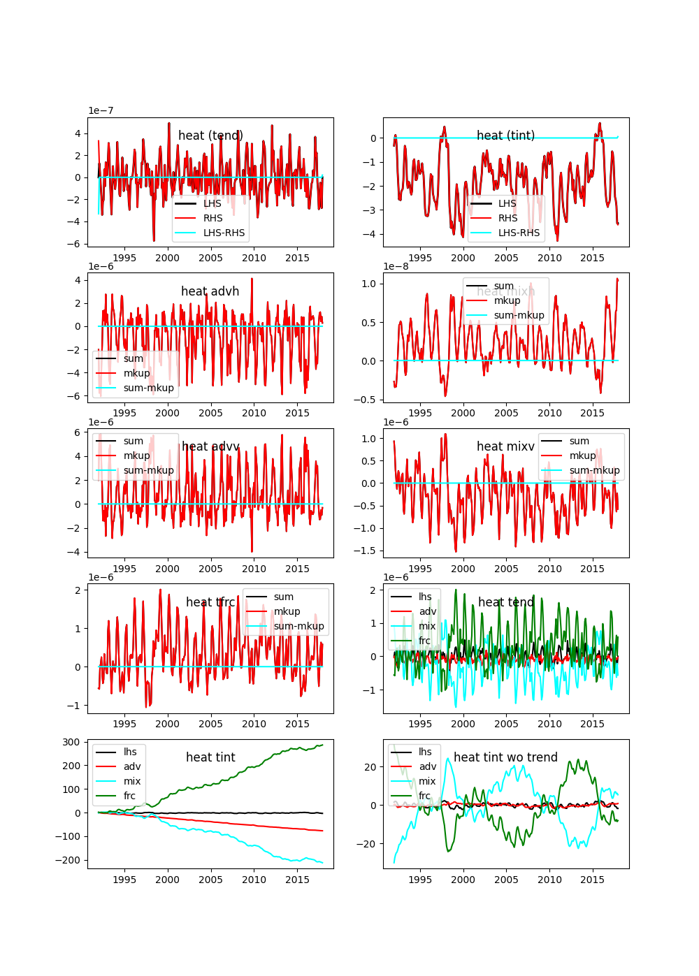
The top two panels show the time series of heat tendency terms (top left) and their time integral (top right). The black, red, and cyan curves represent the terms from the left-hand side (LHS), the right-hand side (RHS), and the difference, respectively. The difference is zero, confirming that the budget is closed.
Panels [2,1], [2,2], [3,1], [3,2], and [4,1] show contributions due to horizontal advection, horizontal mixing, vertical advection, horizontal mixing, and surface forcing, respectively. The black and red curves use two different methods to compute these contributions. The two methods produce the same results, as the difference (cyan) is zero.
Panel [4,2] shows the heat tendency term (black) and its components, including advection (red), mixing (cyan), and surface forcing (green). Forcing and mixing are the two largest terms. Panels [5,1] and [5,2] are the same as Panel [4,2], but for time integrals. The difference between Panels [5,1] and [5,2] is that the latter does not include the trend. Forcing and mixing are also the two largest terms in Panels [5,1] and [5,2].
Method 2: Argument-based Input#
The detailed steps for Method 2 can be found in budg_viz.ipynb (see Tip above).
Load modules
import sys
sys.path.append('/efs_ecco/ECCO/EMU/emu_userinterface_dir/')
import emu_plot_arg_py as ept
import plot_budg
Invoke Method 2
# Budget Tool
globals_dict = ept.emu_plot(run_name="/efs_ecco/owang/ECCO/EMU/tryout/emu_budg_m_2_-170.0_-120.0_-5.0_5.0_10.0_0.0")
Found file: /efs_ecco/ECCO/EMU/emu_userinterface_dir/emu_env.singularity
EMU Input Files directory: /efs/owang/ECCO/EMU_test/emu_input_dir

Specified directory of EMU run to examine: /efs_ecco/owang/ECCO/EMU/tryout/emu_budg_m_2_-170.0_-120.0_-5.0_5.0_10.0_0.0

Reading /efs_ecco/owang/ECCO/EMU/tryout/emu_budg_m_2_-170.0_-120.0_-5.0_5.0_10.0_0.0

Reading Budget Tool output ...
*********************************************
Read sum of heat budget variables
   budg_tend: tendency time-series (per second)
   budg_tend_name: name of variables in budg_tend
from file /efs_ecco/owang/ECCO/EMU/tryout/emu_budg_m_2_-170.0_-120.0_-5.0_5.0_10.0_0.0/output/emu_budg.sum_tend

*********************************************
Read sum of heat budget variables
   budg_tint: time-integrated tendency time-series
   budg_tint_name: name of variables in budg_tint
from file /efs_ecco/owang/ECCO/EMU/tryout/emu_budg_m_2_-170.0_-120.0_-5.0_5.0_10.0_0.0/output/emu_budg.sum_tint

*********************************************
Read 3D masks emu_budg.msk3d_* that describe the spatial location
and direction (+/- 1) of the converging fluxes budg_mkup.
   budg_msk: list of dictionaries, each describing a 3D mask
      budg_msk[n]["msk"]: name (location) of mask n
      budg_msk[n]["msk_dim"]: dimension of mask n (n3D)
      budg_msk[n]["f_msk"]: weights (direction) of mask n
      budg_msk[n]["i_msk"]: i-index of mask n
      budg_msk[n]["j_msk"]: j-index of mask n
      budg_msk[n]["k_msk"]: k-index of mask n
The number of different masks (dictionaries) is len(budg_msk)

*********************************************
Read converging fluxes from files emu_budg.mkup_*
(budget makeup)
   budg_mkup: list of class objects, each describing a particular flux
      budg_mkup[n].var: name of flux n
      budg_mkup[n].msk: name (location) of corresponding mask
      budg_mkup[n].isum: term in emu_budg.sum_tend that this flux (n) is summed in
      budg_mkup[n].mkup_dim: spatial dimension of budg_mkup[n]["mkup"]
      budg_mkup[n].mkup: flux time-series
   budg_nmkup: number of different fluxes
               Same as len(budg_mkup)


***********************
EMU variables read as global variables in module global_emu_var (emu); e.g., emu.nx
***********************
budg_mkup           budg_msk            budg_nmkup          budg_tend
budg_tend_name      budg_tint           budg_tint_name      cs
drc                 drf                 dvol3d              dxc
dxg                 dyc                 dyg                 hfacc
hfacs               hfacw               nr                  nx
ny                  rac                 ras                 raw
raz                 rc                  rf                  sn
xc                  xg                  yc                  yg
Extract Data from Return Dictionary
return_vars_dict = globals_dict.get('return_vars')
Make plot
tt = return_vars_dict['time_values']
lhs_tend = return_vars_dict['lhs_tendency']
rhs_tend = return_vars_dict['rhs_tendency']
lhs_tint = return_vars_dict['lhs_tendency_time_integral']
rhs_tint = return_vars_dict['rhs_tendency_time_integral']
emu_tend = return_vars_dict['emu_tend']
adv_tend = return_vars_dict['adv_tendency']
mix_tend = return_vars_dict['mix_tendency']
frc_tend = return_vars_dict['frc_tendency']
adv_tint = return_vars_dict['adv_tendency_time_integral']
mix_tint = return_vars_dict['mix_tendency_time_integral']
frc_tint = return_vars_dict['frc_tendency_time_integral']
budg_mkup = return_vars_dict['list_flux_obj']
nvar = return_vars_dict['total_num_var']
fbudg = return_vars_dict['budg_quantity']
ibud = return_vars_dict['budg_quantity_idx']
nmonths = return_vars_dict['num_months']
emu_tend_name = return_vars_dict['budg_tend_name']
nmkup = return_vars_dict['num_flux']

# Create the figure
plot_budg.create_budg_fig(tt, lhs_tend, rhs_tend, lhs_tint, rhs_tint, emu_tend, \
            adv_tend, mix_tend, frc_tend, \
            adv_tint, mix_tint, frc_tint, \
                budg_mkup, \
                    nvar, fbudg, ibud, nmonths, emu_tend_name, \
                        nmkup)
Method 2 generates the same figure (not shown; see the second figure embedded in budg_viz.ipynb) as that generated by Method 1.