The ecco_access modules: a starting point for accessing ECCO output on PO.DAAC

Andrew Delman, updated 2025-05-18

Introduction
Importing ecco_access to your workspace
Using the ecco_podaac_to_xrdataset function
Using the ecco_podaac_access function
Accessing ECCOv4 release 5 output

Introduction

In the past several years since ECCOv4 release 4 output was made available on the Physical Oceanography Distributed Active Archive Center or PO.DAAC, a number of Python scripts/functions have been written to facilitate requests of this output, authored by Jack McNelis, Ian Fenty, and Andrew Delman. These codes have been consolidated into the ecco_access modules, in order to standardize the format of the requests.

Note

As of April 2025, the ecco_access modules are included in the ecco_v4_py Python package. There should no longer be a need to clone the ECCO-v4-Python-Tutorial repo to use these tools. Instead, you should clone the ECCOv4-py repo that contains ecco_v4_py, as described below.

This tutorial will help you to start using the ecco_access library, which is comprised of a set of Python modules. Here we introduce the two top-level functions in ecco_access:

• ecco_podaac_to_xrdataset: takes as input a text query or ECCO dataset identifier, and returns an xarray Dataset

• ecco_podaac_access: takes the same input, but returns the URLs/paths or local files where the data is located

Importing ecco_access to your workspace

As of the latest update (April 2025), ecco_access modules are included in ecco_v4_py. To use them, you will need the latest version of ecco_v4_py (1.7.4.1 or later) which is not yet available through conda-forge or Anaconda channels. It is available through pypi, which means that on your local machine or anywhere else you can just run python -m pip install -U ecco_v4_py in your conda environment to install the latest version.

However…the Docker image that is used when launching our OSS servers does not have ecco_v4_py pre-installed. If you run the pip install command above, it will install ecco_v4_py temporarily, but then the next time you start an OSS server (which you will probably do at least once daily during the summer school) it will revert to only what was pre-installed in the Docker image.

One way around this is to clone the repository containing ecco_v4_py into your home directory filesystem on OSS (which is preserved when you start a new server). And then tell your Python notebooks and code to use the version in the cloned repository, rather than the version in the default path for packages.

To do this, open up a terminal window in OSS. Then navigate to your home directory and git clone the ECCOv4-py repository that contains ecco_v4_py:

cd ~
git clone https://github.com/ECCO-GROUP/ECCOv4-py.git

Or if you have a Github SSH key, instead of the 2nd line above you could use git clone git@github.com:ECCO-GROUP/ECCOv4-py.git.

Now that you have the repository with the newer ecco_v4_py, you should have these lines of Python code near the beginning of each notebook when using the ecco_access utilities:

from os.path import join,expanduser
import sys
sys.path.insert(0,join(expanduser('~'),'ECCOv4-py'))
import ecco_v4_py.ecco_access as ea

Note

You can also import ecco_access into your workspace just by importing ecco_v4_py rather than ecco_v4_py.ecco_access. The high-level functions discussed below should work either way. Importing ecco_v4_py.ecco_access is just a little more direct, especially if you are only using the access-related functions of ecco_v4_py.

Using the ecco_podaac_to_xrdataset function

Perhaps the most convenient way to use ecco_access is the ecco_podaac_to_xrdataset; it takes as input a query consisting of NASA Earthdata dataset ShortName(s), ECCO variables, or text strings in the variable descriptions, and outputs an xarray Dataset. Let’s look at the syntax:

import xarray as xr
import matplotlib.pyplot as plt

# tell Python to use the ecco_v4_py in the 'ECCOv4-py' repository, rather than the pre-installed older version
from os.path import join,expanduser
import sys
sys.path.insert(0,join(expanduser('~'),'ECCOv4-py'))

import ecco_v4_py as ecco
import ecco_v4_py.ecco_access as ea

# identify user's home directory
user_home_dir = expanduser('~')

help(ea.ecco_podaac_to_xrdataset)

Help on function ecco_podaac_to_xrdataset in module ecco_v4_py.ecco_access:

ecco_podaac_to_xrdataset(query, version='v4r4', grid=None, time_res='all', StartDate=None, EndDate=None, snapshot_interval=None, mode='download_ifspace', download_root_dir=None, **kwargs)
    This function queries and accesses ECCO datasets from PO.DAAC. The core query and download functions
    are adapted from Jupyter notebooks created by Jack McNelis and Ian Fenty
    (https://github.com/ECCO-GROUP/ECCO-ACCESS/blob/master/PODAAC/Downloading_ECCO_datasets_from_PODAAC/README.md)
    and modified by Andrew Delman (https://ecco-v4-python-tutorial.readthedocs.io).
    It is similar to ecco_podaac_access, except instead of a list of URLs or files,
    an xarray Dataset with all of the queried ECCO datasets is returned.

    Parameters
    ----------
    query: str, list, or dict, defines datasets or variables to access.
           If query is str, it specifies either a dataset ShortName (if query
           matches a NASA Earthdata ShortName), or a text string that can be
           used to search the ECCO ShortNames, variable names, and descriptions.
           A query may also be a list of multiple ShortNames and/or text searches,
           or a dict that contains grid,time_res specifiers as keys and ShortNames
           or text searches as values, e.g.,
           {'native,monthly':['ECCO_L4_SSH_LLC0090GRID_MONTHLY_V4R4',
                              'THETA']}
           will query the native grid monthly SSH datasets, and all native grid
           monthly datasets with variables or descriptions matching 'THETA'.

    version: ('v4r4','v4r5'), specifies ECCO version to query.
             Currently 'v4r5' only works with ['s3_open','s3_get','s3_get_ifspace'] modes,
             or if the files are already stored in download_root_dir/ShortName/.
             Otherwise an error is returned.

    grid: ('native','latlon',None), specifies whether to query datasets with output
          on the native grid or the interpolated lat/lon grid.
          The default None will query both types of grids, unless specified
          otherwise in a query dict (e.g., the example above).

    time_res: ('monthly','daily','snapshot','all'), specifies which time resolution
              to include in query and downloads. 'all' includes all time resolutions,
              and datasets that have no time dimension, such as the grid parameter
              and mixing coefficient datasets.


    StartDate,EndDate: str, in 'YYYY', 'YYYY-MM', or 'YYYY-MM-DD' format,
                       define date range [StartDate,EndDate] for download.
                       EndDate is included in the time range (unlike typical Python ranges).
                       Full ECCOv4r4 date range (default) is '1992-01-01' to '2017-12-31'.
                       For 'SNAPSHOT' datasets, an additional day is added to EndDate to enable
                       closed budgets within the specified date range.

    snapshot_interval: ('monthly', 'daily', or None), if snapshot datasets are included in ShortNames,
                       this determines whether snapshots are included for only the beginning/end
                       of each month ('monthly'), or for every day ('daily').
                       If None or not specified, defaults to 'daily' if any daily mean ShortNames
                       are included and 'monthly' otherwise.

    mode: str, one of the following:
          'download': Download datasets using NASA Earthdata URLs
          'download_ifspace': Check storage availability before downloading.
                              Download only if storage footprint of downloads
                              <= max_avail_frac*(available storage)
          'download_subset': Download spatial and temporal subsets of datasets
                             via Opendap; query help(ecco_access.ecco_podaac_download_subset)
                             to see keyword arguments that can be used in this mode.
          The following modes work within the AWS cloud only:
          's3_open': Access datasets on S3 without downloading.
          's3_open_fsspec': Use json files (generated with `fsspec` and `kerchunk`)
                            for expedited opening of datasets.
          's3_get': Download from S3 (to AWS EC2 instance).
          's3_get_ifspace': Check storage availability before downloading;
                            download if storage footprint
                            <= max_avail_frac*(available storage).
                            Otherwise data are opened "remotely" from S3 bucket.

    download_root_dir: str, defines parent directory to download files to.
                       Files will be downloaded to directory download_root_dir/ShortName/.
                       If not specified, parent directory defaults to '~/Downloads/ECCO_V4r4_PODAAC/',
                       or '~/Downloads/ECCO_V4r5_PODAAC/' if version == 'v4r5'.

    Additional keyword arguments*:
    *This is not an exhaustive list, especially for
    'download_subset' mode; use help(ecco_access.ecco_podaac_download_subset) to display
    options specific to that mode

    max_avail_frac: float, maximum fraction of remaining available disk space to
                    use in storing ECCO datasets.
                    If storing the datasets exceeds this fraction, an error is returned.
                    Valid range is [0,0.9]. If number provided is outside this range, it is replaced
                    by the closer endpoint of the range.

    jsons_root_dir: str, for s3_open_fsspec mode only, the root/parent directory where the
                    fsspec/kerchunk-generated jsons are found.
                    jsons are generated using the steps described here:
                    https://medium.com/pangeo/fake-it-until-you-make-it-reading-goes-netcdf4-data-on-aws-s3
                    as-zarr-for-rapid-data-access-61e33f8fe685.
                    If None (default), jsons_root_dir will be set to ~/MZZ/{version}/.
                    The jsons need to be stored in the following directories/formats:
                    For v4r4: {jsons_root_dir}/MZZ_{GRIDTYPE}_{TIME_RES}/{SHORTNAME}.json.
                    GRIDTYPE is '05DEG' or 'LLC0090GRID' for v4r4;
                    TIME_RES is one of: ('MONTHLY','DAILY','SNAPSHOT','GEOMETRY','MIXING_COEFFS').
                    For v4r5: {jsons_root_dir}/MZZ_{TIME_RES}_{GRIDTYPE}/{SHORTNAME_core}_{TIME_RES}_{GRIDTYPE}_llc090_ECCOV4r5.json.
                    TIME_RES is one of: ('mon_mean','day_mean','snap');
                    GRIDTYPE is one of: ('native','latlon').
                    The SHORTNAME_core is the SHORTNAME without the 'ECCO_L4_' at the beginning,
                    or the grid/time/version IDs at the end (e.g., 'LLC0090GRID_MONTHLY_V4R5').

    jsons_retrieve: bool, if True (default), and jsons are not already stored in jsons_root_dir,
                    retrieve from S3 bucket and store locally in jsons_root_dir.
                    If False, and jsons are not stored in jsons_root_dir,
                    the data retrieval will fail.

    n_workers: int, number of workers to use in concurrent downloads. Benefits typically taper off above 5-6.

    force_redownload: bool, if True, existing files will be redownloaded and replaced;
                            if False (default), existing files will not be replaced.

    show_noredownload_msg: bool, if True (default), and force_redownload=False,
                               display message for each file that is already
                               downloaded (and therefore not re-downloaded);
                               if False, these messages are not shown.

    prompt_request_payer: bool, if True (default), user is prompted to approve
                                (by entering "y" or "Y") any access to a
                                requester pays bucket, otherwise request is canceled;
                                if False, data access proceeds without prompting.

    Returns
    -------
    ds_out: xarray Dataset or dict of xarray Datasets (with ShortNames as keys),
            containing all of the accessed datasets.
            This function does not work with the query modes: 'ls','query','s3_ls','s3_query'.

There are a lot of options that you can use to “submit” a query with this function. Let’s consider a simple case, where we already have the ShortName for the monthly native grid SSH from ECCOv4r4 (ECCO_L4_SSH_LLC0090GRID_MONTHLY_V4R4), and we want to access output from the year 2017. The ShortName goes in the query field, and we can specify start and end dates (in YYYY-MM or YYYY-MM-DD format). The other options that matter most for this request are the mode, and depending on the mode, the download_root_dir or the jsons_root_dir.

Direct download over the internet (mode = ‘download’)

Let’s try the download mode, which retrieves the data over the Internet using NASA Earthdata URLs (this should work on any machine with Internet access, including cloud environments):

# download data and open xarray dataset
curr_shortname = 'ECCO_L4_SSH_LLC0090GRID_MONTHLY_V4R4'
ds_SSH = ea.ecco_podaac_to_xrdataset(curr_shortname,\
                                        StartDate='2017-01',EndDate='2017-12',\
                                        mode='download',\
                                        download_root_dir=join(user_home_dir,'Downloads','ECCO_V4r4_PODAAC'))

Creating download directory /home/jovyan/Downloads/ECCO_V4r4_PODAAC/ECCO_L4_SSH_LLC0090GRID_MONTHLY_V4R4
DL Progress: 100%|#########################| 12/12 [00:04<00:00,  2.52it/s]

=====================================
total downloaded: 71.02 Mb
avg download speed: 14.79 Mb/s
Time spent = 4.803034782409668 seconds

We specified a root directory for the download (which also happens to be the default setting), and the data files are then placed under download_root_dir / ShortName. We can verify that the contents of the file are what we queried:

ds_SSH

<xarray.Dataset> Size: 25MB
Dimensions:    (time: 12, tile: 13, j: 90, i: 90, i_g: 90, j_g: 90, nv: 2, nb: 4)
Coordinates: (12/13)
  * i          (i) int32 360B 0 1 2 3 4 5 6 7 8 9 ... 81 82 83 84 85 86 87 88 89
  * i_g        (i_g) int32 360B 0 1 2 3 4 5 6 7 8 ... 81 82 83 84 85 86 87 88 89
  * j          (j) int32 360B 0 1 2 3 4 5 6 7 8 9 ... 81 82 83 84 85 86 87 88 89
  * j_g        (j_g) int32 360B 0 1 2 3 4 5 6 7 8 ... 81 82 83 84 85 86 87 88 89
  * tile       (tile) int32 52B 0 1 2 3 4 5 6 7 8 9 10 11 12
  * time       (time) datetime64[ns] 96B 2017-01-16T12:00:00 ... 2017-12-16T0...
    ...         ...
    YC         (tile, j, i) float32 421kB dask.array<chunksize=(13, 90, 90), meta=np.ndarray>
    XG         (tile, j_g, i_g) float32 421kB dask.array<chunksize=(13, 90, 90), meta=np.ndarray>
    YG         (tile, j_g, i_g) float32 421kB dask.array<chunksize=(13, 90, 90), meta=np.ndarray>
    time_bnds  (time, nv) datetime64[ns] 192B dask.array<chunksize=(1, 2), meta=np.ndarray>
    XC_bnds    (tile, j, i, nb) float32 2MB dask.array<chunksize=(13, 90, 90, 4), meta=np.ndarray>
    YC_bnds    (tile, j, i, nb) float32 2MB dask.array<chunksize=(13, 90, 90, 4), meta=np.ndarray>
Dimensions without coordinates: nv, nb
Data variables:
    SSH        (time, tile, j, i) float32 5MB dask.array<chunksize=(1, 13, 90, 90), meta=np.ndarray>
    SSHIBC     (time, tile, j, i) float32 5MB dask.array<chunksize=(1, 13, 90, 90), meta=np.ndarray>
    SSHNOIBC   (time, tile, j, i) float32 5MB dask.array<chunksize=(1, 13, 90, 90), meta=np.ndarray>
    ETAN       (time, tile, j, i) float32 5MB dask.array<chunksize=(1, 13, 90, 90), meta=np.ndarray>
Attributes: (12/57)
    acknowledgement:              This research was carried out by the Jet Pr...
    author:                       Ian Fenty and Ou Wang
    cdm_data_type:                Grid
    comment:                      Fields provided on the curvilinear lat-lon-...
    Conventions:                  CF-1.8, ACDD-1.3
    coordinates_comment:          Note: the global 'coordinates' attribute de...
    ...                           ...
    time_coverage_duration:       P1M
    time_coverage_end:            2017-02-01T00:00:00
    time_coverage_resolution:     P1M
    time_coverage_start:          2017-01-01T00:00:00
    title:                        ECCO Sea Surface Height - Monthly Mean llc9...
    uuid:                         a21a5c30-400c-11eb-a9e0-0cc47a3f49c3

xarray.Dataset

• Dimensions:
  • time: 12
  • tile: 13
  • j: 90
  • i: 90
  • i_g: 90
  • j_g: 90
  • nv: 2
  • nb: 4
• Coordinates: (13)
  • i
    (i)
    int32
    0 1 2 3 4 5 6 ... 84 85 86 87 88 89

    axis :

    X

    long_name :

    grid index in x for variables at tracer and 'v' locations

    swap_dim :

    XC

    comment :

    In the Arakawa C-grid system, tracer (e.g., THETA) and 'v' variables (e.g., VVEL) have the same x coordinate on the model grid.

    coverage_content_type :

    coordinate

    array([ 0,  1,  2,  3,  4,  5,  6,  7,  8,  9, 10, 11, 12, 13, 14, 15, 16, 17,
           18, 19, 20, 21, 22, 23, 24, 25, 26, 27, 28, 29, 30, 31, 32, 33, 34, 35,
           36, 37, 38, 39, 40, 41, 42, 43, 44, 45, 46, 47, 48, 49, 50, 51, 52, 53,
           54, 55, 56, 57, 58, 59, 60, 61, 62, 63, 64, 65, 66, 67, 68, 69, 70, 71,
           72, 73, 74, 75, 76, 77, 78, 79, 80, 81, 82, 83, 84, 85, 86, 87, 88, 89],
          dtype=int32)

  • i_g
    (i_g)
    int32
    0 1 2 3 4 5 6 ... 84 85 86 87 88 89

    axis :

    X

    long_name :

    grid index in x for variables at 'u' and 'g' locations

    c_grid_axis_shift :

    -0.5

    swap_dim :

    XG

    comment :

    In the Arakawa C-grid system, 'u' (e.g., UVEL) and 'g' variables (e.g., XG) have the same x coordinate on the model grid.

    coverage_content_type :

    coordinate

    array([ 0,  1,  2,  3,  4,  5,  6,  7,  8,  9, 10, 11, 12, 13, 14, 15, 16, 17,
           18, 19, 20, 21, 22, 23, 24, 25, 26, 27, 28, 29, 30, 31, 32, 33, 34, 35,
           36, 37, 38, 39, 40, 41, 42, 43, 44, 45, 46, 47, 48, 49, 50, 51, 52, 53,
           54, 55, 56, 57, 58, 59, 60, 61, 62, 63, 64, 65, 66, 67, 68, 69, 70, 71,
           72, 73, 74, 75, 76, 77, 78, 79, 80, 81, 82, 83, 84, 85, 86, 87, 88, 89],
          dtype=int32)

  • j
    (j)
    int32
    0 1 2 3 4 5 6 ... 84 85 86 87 88 89

    axis :

    Y

    long_name :

    grid index in y for variables at tracer and 'u' locations

    swap_dim :

    YC

    comment :

    In the Arakawa C-grid system, tracer (e.g., THETA) and 'u' variables (e.g., UVEL) have the same y coordinate on the model grid.

    coverage_content_type :

    coordinate

    array([ 0,  1,  2,  3,  4,  5,  6,  7,  8,  9, 10, 11, 12, 13, 14, 15, 16, 17,
           18, 19, 20, 21, 22, 23, 24, 25, 26, 27, 28, 29, 30, 31, 32, 33, 34, 35,
           36, 37, 38, 39, 40, 41, 42, 43, 44, 45, 46, 47, 48, 49, 50, 51, 52, 53,
           54, 55, 56, 57, 58, 59, 60, 61, 62, 63, 64, 65, 66, 67, 68, 69, 70, 71,
           72, 73, 74, 75, 76, 77, 78, 79, 80, 81, 82, 83, 84, 85, 86, 87, 88, 89],
          dtype=int32)

  • j_g
    (j_g)
    int32
    0 1 2 3 4 5 6 ... 84 85 86 87 88 89

    axis :

    Y

    long_name :

    grid index in y for variables at 'v' and 'g' locations

    c_grid_axis_shift :

    -0.5

    swap_dim :

    YG

    comment :

    In the Arakawa C-grid system, 'v' (e.g., VVEL) and 'g' variables (e.g., XG) have the same y coordinate.

    coverage_content_type :

    coordinate

    array([ 0,  1,  2,  3,  4,  5,  6,  7,  8,  9, 10, 11, 12, 13, 14, 15, 16, 17,
           18, 19, 20, 21, 22, 23, 24, 25, 26, 27, 28, 29, 30, 31, 32, 33, 34, 35,
           36, 37, 38, 39, 40, 41, 42, 43, 44, 45, 46, 47, 48, 49, 50, 51, 52, 53,
           54, 55, 56, 57, 58, 59, 60, 61, 62, 63, 64, 65, 66, 67, 68, 69, 70, 71,
           72, 73, 74, 75, 76, 77, 78, 79, 80, 81, 82, 83, 84, 85, 86, 87, 88, 89],
          dtype=int32)

  • tile
    (tile)
    int32
    0 1 2 3 4 5 6 7 8 9 10 11 12

    long_name :

    lat-lon-cap tile index

    comment :

    The ECCO V4 horizontal model grid is divided into 13 tiles of 90x90 cells for convenience.

    coverage_content_type :

    coordinate

    array([ 0,  1,  2,  3,  4,  5,  6,  7,  8,  9, 10, 11, 12], dtype=int32)

  • time
    (time)
    datetime64[ns]
    2017-01-16T12:00:00 ... 2017-12-...

    long_name :

    center time of averaging period

    axis :

    T

    bounds :

    time_bnds

    coverage_content_type :

    coordinate

    standard_name :

    time

    array(['2017-01-16T12:00:00.000000000', '2017-02-15T00:00:00.000000000',
           '2017-03-16T12:00:00.000000000', '2017-04-16T00:00:00.000000000',
           '2017-05-16T12:00:00.000000000', '2017-06-16T00:00:00.000000000',
           '2017-07-16T12:00:00.000000000', '2017-08-16T12:00:00.000000000',
           '2017-09-16T00:00:00.000000000', '2017-10-16T12:00:00.000000000',
           '2017-11-16T00:00:00.000000000', '2017-12-16T06:00:00.000000000'],
          dtype='datetime64[ns]')

  • XC
    (tile, j, i)
    float32
    dask.array<chunksize=(13, 90, 90), meta=np.ndarray>

    long_name :

    longitude of tracer grid cell center

    units :

    degrees_east

    coordinate :

    YC XC

    bounds :

    XC_bnds

    comment :

    nonuniform grid spacing

    coverage_content_type :

    coordinate

    standard_name :

    longitude

    Array Chunk Bytes 411.33 kiB 411.33 kiB Shape (13, 90, 90) (13, 90, 90) Dask graph 1 chunks in 2 graph layers Data type float32 numpy.ndarray

  • YC
    (tile, j, i)
    float32
    dask.array<chunksize=(13, 90, 90), meta=np.ndarray>

    long_name :

    latitude of tracer grid cell center

    units :

    degrees_north

    coordinate :

    YC XC

    bounds :

    YC_bnds

    comment :

    nonuniform grid spacing

    coverage_content_type :

    coordinate

    standard_name :

    latitude

    Array Chunk Bytes 411.33 kiB 411.33 kiB Shape (13, 90, 90) (13, 90, 90) Dask graph 1 chunks in 2 graph layers Data type float32 numpy.ndarray

  • XG
    (tile, j_g, i_g)
    float32
    dask.array<chunksize=(13, 90, 90), meta=np.ndarray>

    long_name :

    longitude of 'southwest' corner of tracer grid cell

    units :

    degrees_east

    coordinate :

    YG XG

    comment :

    Nonuniform grid spacing. Note: 'southwest' does not correspond to geographic orientation but is used for convenience to describe the computational grid. See MITgcm dcoumentation for details.

    coverage_content_type :

    coordinate

    standard_name :

    longitude

    Array Chunk Bytes 411.33 kiB 411.33 kiB Shape (13, 90, 90) (13, 90, 90) Dask graph 1 chunks in 2 graph layers Data type float32 numpy.ndarray

  • YG
    (tile, j_g, i_g)
    float32
    dask.array<chunksize=(13, 90, 90), meta=np.ndarray>

    long_name :

    latitude of 'southwest' corner of tracer grid cell

    units :

    degrees_north

    coordinate :

    YG XG

    comment :

    Nonuniform grid spacing. Note: 'southwest' does not correspond to geographic orientation but is used for convenience to describe the computational grid. See MITgcm dcoumentation for details.

    coverage_content_type :

    coordinate

    standard_name :

    latitude

    Array Chunk Bytes 411.33 kiB 411.33 kiB Shape (13, 90, 90) (13, 90, 90) Dask graph 1 chunks in 2 graph layers Data type float32 numpy.ndarray

  • time_bnds
    (time, nv)
    datetime64[ns]
    dask.array<chunksize=(1, 2), meta=np.ndarray>

    comment :

    Start and end times of averaging period.

    coverage_content_type :

    coordinate

    long_name :

    time bounds of averaging period

    Array Chunk Bytes 192 B 16 B Shape (12, 2) (1, 2) Dask graph 12 chunks in 25 graph layers Data type datetime64[ns] numpy.ndarray

  • XC_bnds
    (tile, j, i, nb)
    float32
    dask.array<chunksize=(13, 90, 90, 4), meta=np.ndarray>

    comment :

    Bounds array follows CF conventions. XC_bnds[i,j,0] = 'southwest' corner (j-1, i-1), XC_bnds[i,j,1] = 'southeast' corner (j-1, i+1), XC_bnds[i,j,2] = 'northeast' corner (j+1, i+1), XC_bnds[i,j,3] = 'northwest' corner (j+1, i-1). Note: 'southwest', 'southeast', northwest', and 'northeast' do not correspond to geographic orientation but are used for convenience to describe the computational grid. See MITgcm dcoumentation for details.

    coverage_content_type :

    coordinate

    long_name :

    longitudes of tracer grid cell corners

    Array Chunk Bytes 1.61 MiB 1.61 MiB Shape (13, 90, 90, 4) (13, 90, 90, 4) Dask graph 1 chunks in 2 graph layers Data type float32 numpy.ndarray

  • YC_bnds
    (tile, j, i, nb)
    float32
    dask.array<chunksize=(13, 90, 90, 4), meta=np.ndarray>

    comment :

    Bounds array follows CF conventions. YC_bnds[i,j,0] = 'southwest' corner (j-1, i-1), YC_bnds[i,j,1] = 'southeast' corner (j-1, i+1), YC_bnds[i,j,2] = 'northeast' corner (j+1, i+1), YC_bnds[i,j,3] = 'northwest' corner (j+1, i-1). Note: 'southwest', 'southeast', northwest', and 'northeast' do not correspond to geographic orientation but are used for convenience to describe the computational grid. See MITgcm dcoumentation for details.

    coverage_content_type :

    coordinate

    long_name :

    latitudes of tracer grid cell corners

    Array Chunk Bytes 1.61 MiB 1.61 MiB Shape (13, 90, 90, 4) (13, 90, 90, 4) Dask graph 1 chunks in 2 graph layers Data type float32 numpy.ndarray

• Data variables: (4)
  • SSH
    (time, tile, j, i)
    float32
    dask.array<chunksize=(1, 13, 90, 90), meta=np.ndarray>

    long_name :

    Dynamic sea surface height anomaly

    units :

    m

    coverage_content_type :

    modelResult

    standard_name :

    sea_surface_height_above_geoid

    comment :

    Dynamic sea surface height anomaly above the geoid, suitable for comparisons with altimetry sea surface height data products that apply the inverse barometer (IB) correction. Note: SSH is calculated by correcting model sea level anomaly ETAN for three effects: a) global mean steric sea level changes related to density changes in the Boussinesq volume-conserving model (Greatbatch correction, see sterGloH), b) the inverted barometer (IB) effect (see SSHIBC) and c) sea level displacement due to sea-ice and snow pressure loading (see sIceLoad). SSH can be compared with the similarly-named SSH variable in previous ECCO products that did not include atmospheric pressure loading (e.g., Version 4 Release 3). Use SSHNOIBC for comparisons with altimetry data products that do NOT apply the IB correction.

    valid_min :

    -1.8805772066116333

    valid_max :

    1.4207719564437866

    Array Chunk Bytes 4.82 MiB 411.33 kiB Shape (12, 13, 90, 90) (1, 13, 90, 90) Dask graph 12 chunks in 25 graph layers Data type float32 numpy.ndarray

  • SSHIBC
    (time, tile, j, i)
    float32
    dask.array<chunksize=(1, 13, 90, 90), meta=np.ndarray>

    long_name :

    The inverted barometer (IB) correction to sea surface height due to atmospheric pressure loading

    units :

    m

    coverage_content_type :

    modelResult

    comment :

    Not an SSH itself, but a correction to model sea level anomaly (ETAN) required to account for the static part of sea surface displacement by atmosphere pressure loading: SSH = SSHNOIBC - SSHIBC. Note: Use SSH for model-data comparisons with altimetry data products that DO apply the IB correction and SSHNOIBC for comparisons with altimetry data products that do NOT apply the IB correction.

    valid_min :

    -0.30144819617271423

    valid_max :

    0.5248842239379883

    Array Chunk Bytes 4.82 MiB 411.33 kiB Shape (12, 13, 90, 90) (1, 13, 90, 90) Dask graph 12 chunks in 25 graph layers Data type float32 numpy.ndarray

  • SSHNOIBC
    (time, tile, j, i)
    float32
    dask.array<chunksize=(1, 13, 90, 90), meta=np.ndarray>

    long_name :

    Sea surface height anomaly without the inverted barometer (IB) correction

    units :

    m

    coverage_content_type :

    modelResult

    comment :

    Sea surface height anomaly above the geoid without the inverse barometer (IB) correction, suitable for comparisons with altimetry sea surface height data products that do NOT apply the inverse barometer (IB) correction. Note: SSHNOIBC is calculated by correcting model sea level anomaly ETAN for two effects: a) global mean steric sea level changes related to density changes in the Boussinesq volume-conserving model (Greatbatch correction, see sterGloH), b) sea level displacement due to sea-ice and snow pressure loading (see sIceLoad). In ECCO Version 4 Release 4 the model is forced with atmospheric pressure loading. SSHNOIBC does not correct for the static part of the effect of atmosphere pressure loading on sea surface height (the so-called inverse barometer (IB) correction). Use SSH for comparisons with altimetry data products that DO apply the IB correction.

    valid_min :

    -1.6654272079467773

    valid_max :

    1.4550364017486572

    Array Chunk Bytes 4.82 MiB 411.33 kiB Shape (12, 13, 90, 90) (1, 13, 90, 90) Dask graph 12 chunks in 25 graph layers Data type float32 numpy.ndarray

  • ETAN
    (time, tile, j, i)
    float32
    dask.array<chunksize=(1, 13, 90, 90), meta=np.ndarray>

    long_name :

    Model sea level anomaly

    units :

    m

    coverage_content_type :

    modelResult

    comment :

    Model sea level anomaly WITHOUT corrections for global mean density (steric) changes, inverted barometer effect, or volume displacement due to submerged sea-ice and snow . Note: ETAN should NOT be used for comparisons with altimetry data products because ETAN is NOT corrected for (a) global mean steric sea level changes related to density changes in the Boussinesq volume-conserving model (Greatbatch correction, see sterGloH) nor (b) sea level displacement due to submerged sea-ice and snow (see sIceLoad). These corrections ARE made for the variables SSH and SSHNOIBC.

    valid_min :

    -8.304216384887695

    valid_max :

    1.460192084312439

    Array Chunk Bytes 4.82 MiB 411.33 kiB Shape (12, 13, 90, 90) (1, 13, 90, 90) Dask graph 12 chunks in 25 graph layers Data type float32 numpy.ndarray

• Indexes: (6)
  • i
    PandasIndex

    PandasIndex(Index([ 0,  1,  2,  3,  4,  5,  6,  7,  8,  9, 10, 11, 12, 13, 14, 15, 16, 17,
           18, 19, 20, 21, 22, 23, 24, 25, 26, 27, 28, 29, 30, 31, 32, 33, 34, 35,
           36, 37, 38, 39, 40, 41, 42, 43, 44, 45, 46, 47, 48, 49, 50, 51, 52, 53,
           54, 55, 56, 57, 58, 59, 60, 61, 62, 63, 64, 65, 66, 67, 68, 69, 70, 71,
           72, 73, 74, 75, 76, 77, 78, 79, 80, 81, 82, 83, 84, 85, 86, 87, 88, 89],
          dtype='int32', name='i'))

  • i_g
    PandasIndex

    PandasIndex(Index([ 0,  1,  2,  3,  4,  5,  6,  7,  8,  9, 10, 11, 12, 13, 14, 15, 16, 17,
           18, 19, 20, 21, 22, 23, 24, 25, 26, 27, 28, 29, 30, 31, 32, 33, 34, 35,
           36, 37, 38, 39, 40, 41, 42, 43, 44, 45, 46, 47, 48, 49, 50, 51, 52, 53,
           54, 55, 56, 57, 58, 59, 60, 61, 62, 63, 64, 65, 66, 67, 68, 69, 70, 71,
           72, 73, 74, 75, 76, 77, 78, 79, 80, 81, 82, 83, 84, 85, 86, 87, 88, 89],
          dtype='int32', name='i_g'))

  • j
    PandasIndex

    PandasIndex(Index([ 0,  1,  2,  3,  4,  5,  6,  7,  8,  9, 10, 11, 12, 13, 14, 15, 16, 17,
           18, 19, 20, 21, 22, 23, 24, 25, 26, 27, 28, 29, 30, 31, 32, 33, 34, 35,
           36, 37, 38, 39, 40, 41, 42, 43, 44, 45, 46, 47, 48, 49, 50, 51, 52, 53,
           54, 55, 56, 57, 58, 59, 60, 61, 62, 63, 64, 65, 66, 67, 68, 69, 70, 71,
           72, 73, 74, 75, 76, 77, 78, 79, 80, 81, 82, 83, 84, 85, 86, 87, 88, 89],
          dtype='int32', name='j'))

  • j_g
    PandasIndex

    PandasIndex(Index([ 0,  1,  2,  3,  4,  5,  6,  7,  8,  9, 10, 11, 12, 13, 14, 15, 16, 17,
           18, 19, 20, 21, 22, 23, 24, 25, 26, 27, 28, 29, 30, 31, 32, 33, 34, 35,
           36, 37, 38, 39, 40, 41, 42, 43, 44, 45, 46, 47, 48, 49, 50, 51, 52, 53,
           54, 55, 56, 57, 58, 59, 60, 61, 62, 63, 64, 65, 66, 67, 68, 69, 70, 71,
           72, 73, 74, 75, 76, 77, 78, 79, 80, 81, 82, 83, 84, 85, 86, 87, 88, 89],
          dtype='int32', name='j_g'))

  • tile
    PandasIndex

    PandasIndex(Index([0, 1, 2, 3, 4, 5, 6, 7, 8, 9, 10, 11, 12], dtype='int32', name='tile'))

  • time
    PandasIndex

    PandasIndex(DatetimeIndex(['2017-01-16 12:00:00', '2017-02-15 00:00:00',
                   '2017-03-16 12:00:00', '2017-04-16 00:00:00',
                   '2017-05-16 12:00:00', '2017-06-16 00:00:00',
                   '2017-07-16 12:00:00', '2017-08-16 12:00:00',
                   '2017-09-16 00:00:00', '2017-10-16 12:00:00',
                   '2017-11-16 00:00:00', '2017-12-16 06:00:00'],
                  dtype='datetime64[ns]', name='time', freq=None))

• Attributes: (57)

  acknowledgement :

  This research was carried out by the Jet Propulsion Laboratory, managed by the California Institute of Technology under a contract with the National Aeronautics and Space Administration.

  author :

  Ian Fenty and Ou Wang

  cdm_data_type :

  Grid

  comment :

  Fields provided on the curvilinear lat-lon-cap 90 (llc90) native grid used in the ECCO model. SSH (dynamic sea surface height) = SSHNOIBC (dynamic sea surface without the inverse barometer correction) - SSHIBC (inverse barometer correction). The inverted barometer correction accounts for variations in sea surface height due to atmospheric pressure variations. Note: ETAN is model sea level anomaly and should not be compared with satellite altimetery products, see SSH and ETAN for more details.

  Conventions :

  CF-1.8, ACDD-1.3

  coordinates_comment :

  Note: the global 'coordinates' attribute describes auxillary coordinates.

  creator_email :

  ecco-group@mit.edu

  creator_institution :

  NASA Jet Propulsion Laboratory (JPL)

  creator_name :

  ECCO Consortium

  creator_type :

  group

  creator_url :

  https://ecco-group.org

  date_created :

  2020-12-16T18:07:36

  date_issued :

  2020-12-16T18:07:36

  date_metadata_modified :

  2021-03-15T21:57:04

  date_modified :

  2021-03-15T21:57:04

  geospatial_bounds_crs :

  EPSG:4326

  geospatial_lat_max :

  90.0

  geospatial_lat_min :

  -90.0

  geospatial_lat_resolution :

  variable

  geospatial_lat_units :

  degrees_north

  geospatial_lon_max :

  180.0

  geospatial_lon_min :

  -180.0

  geospatial_lon_resolution :

  variable

  geospatial_lon_units :

  degrees_east

  history :

  Inaugural release of an ECCO Central Estimate solution to PO.DAAC

  id :

  10.5067/ECL5M-SSH44

  institution :

  NASA Jet Propulsion Laboratory (JPL)

  instrument_vocabulary :

  GCMD instrument keywords

  keywords :

  EARTH SCIENCE > OCEANS > SEA SURFACE TOPOGRAPHY > SEA SURFACE HEIGHT, EARTH SCIENCE SERVICES > MODELS > EARTH SCIENCE REANALYSES/ASSIMILATION MODELS

  keywords_vocabulary :

  NASA Global Change Master Directory (GCMD) Science Keywords

  license :

  Public Domain

  metadata_link :

  https://cmr.earthdata.nasa.gov/search/collections.umm_json?ShortName=ECCO_L4_SSH_LLC0090GRID_MONTHLY_V4R4

  naming_authority :

  gov.nasa.jpl

  platform :

  ERS-1/2, TOPEX/Poseidon, Geosat Follow-On (GFO), ENVISAT, Jason-1, Jason-2, CryoSat-2, SARAL/AltiKa, Jason-3, AVHRR, Aquarius, SSM/I, SSMIS, GRACE, DTU17MDT, Argo, WOCE, GO-SHIP, MEOP, Ice Tethered Profilers (ITP)

  platform_vocabulary :

  GCMD platform keywords

  processing_level :

  L4

  product_name :

  SEA_SURFACE_HEIGHT_mon_mean_2017-01_ECCO_V4r4_native_llc0090.nc

  product_time_coverage_end :

  2018-01-01T00:00:00

  product_time_coverage_start :

  1992-01-01T12:00:00

  product_version :

  Version 4, Release 4

  program :

  NASA Physical Oceanography, Cryosphere, Modeling, Analysis, and Prediction (MAP)

  project :

  Estimating the Circulation and Climate of the Ocean (ECCO)

  publisher_email :

  podaac@podaac.jpl.nasa.gov

  publisher_institution :

  PO.DAAC

  publisher_name :

  Physical Oceanography Distributed Active Archive Center (PO.DAAC)

  publisher_type :

  institution

  publisher_url :

  https://podaac.jpl.nasa.gov

  references :

  ECCO Consortium, Fukumori, I., Wang, O., Fenty, I., Forget, G., Heimbach, P., & Ponte, R. M. 2020. Synopsis of the ECCO Central Production Global Ocean and Sea-Ice State Estimate (Version 4 Release 4). doi:10.5281/zenodo.3765928

  source :

  The ECCO V4r4 state estimate was produced by fitting a free-running solution of the MITgcm (checkpoint 66g) to satellite and in situ observational data in a least squares sense using the adjoint method

  standard_name_vocabulary :

  NetCDF Climate and Forecast (CF) Metadata Convention

  summary :

  This dataset provides monthly-averaged dynamic sea surface height and model sea level anomaly on the lat-lon-cap 90 (llc90) native model grid from the ECCO Version 4 Release 4 (V4r4) ocean and sea-ice state estimate. Estimating the Circulation and Climate of the Ocean (ECCO) state estimates are dynamically and kinematically-consistent reconstructions of the three-dimensional, time-evolving ocean, sea-ice, and surface atmospheric states. ECCO V4r4 is a free-running solution of a global, nominally 1-degree configuration of the MIT general circulation model (MITgcm) that has been fit to observations in a least-squares sense. Observational data constraints used in V4r4 include sea surface height (SSH) from satellite altimeters [ERS-1/2, TOPEX/Poseidon, GFO, ENVISAT, Jason-1,2,3, CryoSat-2, and SARAL/AltiKa]; sea surface temperature (SST) from satellite radiometers [AVHRR], sea surface salinity (SSS) from the Aquarius satellite radiometer/scatterometer, ocean bottom pressure (OBP) from the GRACE satellite gravimeter; sea-ice concentration from satellite radiometers [SSM/I and SSMIS], and in-situ ocean temperature and salinity measured with conductivity-temperature-depth (CTD) sensors and expendable bathythermographs (XBTs) from several programs [e.g., WOCE, GO-SHIP, Argo, and others] and platforms [e.g., research vessels, gliders, moorings, ice-tethered profilers, and instrumented pinnipeds]. V4r4 covers the period 1992-01-01T12:00:00 to 2018-01-01T00:00:00.

  time_coverage_duration :

  P1M

  time_coverage_end :

  2017-02-01T00:00:00

  time_coverage_resolution :

  P1M

  time_coverage_start :

  2017-01-01T00:00:00

  title :

  ECCO Sea Surface Height - Monthly Mean llc90 Grid (Version 4 Release 4)

  uuid :

  a21a5c30-400c-11eb-a9e0-0cc47a3f49c3

In-cloud direct access with pre-generated json files (mode = ‘s3_open_fsspec’)

Now, if you are part of the ECCO Summer School you are also working in a cloud environment which means that you have many more access modes open to you. Let’s try s3_open_fsspec, which opens the files from S3 (no download necessary), and uses json files with the data chunking information to open the files exceptionally fast. This means you need to provide the directory jsons_root_dir where the jsons are located, on the efs_ecco drive: /efs_ecco/mzz-jsons.

curr_shortname = 'ECCO_L4_SSH_LLC0090GRID_MONTHLY_V4R4'
ds_SSH_s3 = ea.ecco_podaac_to_xrdataset(curr_shortname,\
                                        StartDate='2017-01',EndDate='2017-12',\
                                        mode='s3_open_fsspec',\
                                        jsons_root_dir=join('/efs_ecco','mzz-jsons'))

ds_SSH_s3

<xarray.Dataset> Size: 25MB
Dimensions:    (time: 12, tile: 13, j: 90, i: 90, nb: 4, j_g: 90, i_g: 90, nv: 2)
Coordinates: (12/13)
  * time       (time) datetime64[ns] 96B 2017-01-16T12:00:00 ... 2017-12-16T0...
    XC         (tile, j, i) float32 421kB dask.array<chunksize=(13, 90, 90), meta=np.ndarray>
    XC_bnds    (tile, j, i, nb) float32 2MB dask.array<chunksize=(13, 90, 90, 4), meta=np.ndarray>
    XG         (tile, j_g, i_g) float32 421kB dask.array<chunksize=(13, 90, 90), meta=np.ndarray>
    YC         (tile, j, i) float32 421kB dask.array<chunksize=(13, 90, 90), meta=np.ndarray>
    YC_bnds    (tile, j, i, nb) float32 2MB dask.array<chunksize=(13, 90, 90, 4), meta=np.ndarray>
    ...         ...
  * i          (i) int32 360B 0 1 2 3 4 5 6 7 8 9 ... 81 82 83 84 85 86 87 88 89
  * i_g        (i_g) int32 360B 0 1 2 3 4 5 6 7 8 ... 81 82 83 84 85 86 87 88 89
  * j          (j) int32 360B 0 1 2 3 4 5 6 7 8 9 ... 81 82 83 84 85 86 87 88 89
  * j_g        (j_g) int32 360B 0 1 2 3 4 5 6 7 8 ... 81 82 83 84 85 86 87 88 89
  * tile       (tile) int32 52B 0 1 2 3 4 5 6 7 8 9 10 11 12
    time_bnds  (time, nv) datetime64[ns] 192B dask.array<chunksize=(12, 2), meta=np.ndarray>
Dimensions without coordinates: nb, nv
Data variables:
    ETAN       (time, tile, j, i) float32 5MB dask.array<chunksize=(4, 13, 90, 90), meta=np.ndarray>
    SSH        (time, tile, j, i) float32 5MB dask.array<chunksize=(4, 13, 90, 90), meta=np.ndarray>
    SSHIBC     (time, tile, j, i) float32 5MB dask.array<chunksize=(4, 13, 90, 90), meta=np.ndarray>
    SSHNOIBC   (time, tile, j, i) float32 5MB dask.array<chunksize=(4, 13, 90, 90), meta=np.ndarray>
Attributes: (12/57)
    Conventions:                  CF-1.8, ACDD-1.3
    acknowledgement:              This research was carried out by the Jet Pr...
    author:                       Ian Fenty and Ou Wang
    cdm_data_type:                Grid
    comment:                      Fields provided on the curvilinear lat-lon-...
    coordinates_comment:          Note: the global 'coordinates' attribute de...
    ...                           ...
    time_coverage_duration:       P1M
    time_coverage_end:            1992-02-01T00:00:00
    time_coverage_resolution:     P1M
    time_coverage_start:          1992-01-01T12:00:00
    title:                        ECCO Sea Surface Height - Monthly Mean llc9...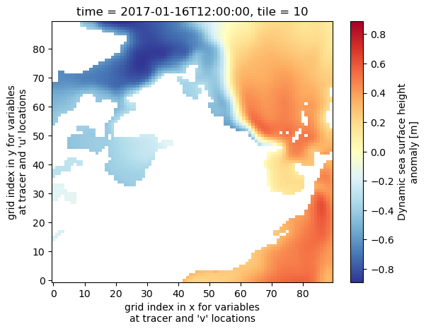
    uuid:                         9302811e-400c-11eb-b69e-0cc47a3f49c3

xarray.Dataset

• Dimensions:
  • time: 12
  • tile: 13
  • j: 90
  • i: 90
  • nb: 4
  • j_g: 90
  • i_g: 90
  • nv: 2
• Coordinates: (13)
  • time
    (time)
    datetime64[ns]
    2017-01-16T12:00:00 ... 2017-12-...

    axis :

    T

    bounds :

    time_bnds

    coverage_content_type :

    coordinate

    long_name :

    center time of averaging period

    standard_name :

    time

    array(['2017-01-16T12:00:00.000000000', '2017-02-15T00:00:00.000000000',
           '2017-03-16T12:00:00.000000000', '2017-04-16T00:00:00.000000000',
           '2017-05-16T12:00:00.000000000', '2017-06-16T00:00:00.000000000',
           '2017-07-16T12:00:00.000000000', '2017-08-16T12:00:00.000000000',
           '2017-09-16T00:00:00.000000000', '2017-10-16T12:00:00.000000000',
           '2017-11-16T00:00:00.000000000', '2017-12-16T06:00:00.000000000'],
          dtype='datetime64[ns]')

  • XC
    (tile, j, i)
    float32
    dask.array<chunksize=(13, 90, 90), meta=np.ndarray>

    bounds :

    XC_bnds

    comment :

    nonuniform grid spacing

    coordinate :

    YC XC

    coverage_content_type :

    coordinate

    long_name :

    longitude of tracer grid cell center

    standard_name :

    longitude

    units :

    degrees_east

    Array Chunk Bytes 411.33 kiB 411.33 kiB Shape (13, 90, 90) (13, 90, 90) Dask graph 1 chunks in 2 graph layers Data type float32 numpy.ndarray

  • XC_bnds
    (tile, j, i, nb)
    float32
    dask.array<chunksize=(13, 90, 90, 4), meta=np.ndarray>

    comment :

    Bounds array follows CF conventions. XC_bnds[i,j,0] = 'southwest' corner (j-1, i-1), XC_bnds[i,j,1] = 'southeast' corner (j-1, i+1), XC_bnds[i,j,2] = 'northeast' corner (j+1, i+1), XC_bnds[i,j,3] = 'northwest' corner (j+1, i-1). Note: 'southwest', 'southeast', northwest', and 'northeast' do not correspond to geographic orientation but are used for convenience to describe the computational grid. See MITgcm dcoumentation for details.

    coverage_content_type :

    coordinate

    long_name :

    longitudes of tracer grid cell corners

    Array Chunk Bytes 1.61 MiB 1.61 MiB Shape (13, 90, 90, 4) (13, 90, 90, 4) Dask graph 1 chunks in 2 graph layers Data type float32 numpy.ndarray

  • XG
    (tile, j_g, i_g)
    float32
    dask.array<chunksize=(13, 90, 90), meta=np.ndarray>

    comment :

    Nonuniform grid spacing. Note: 'southwest' does not correspond to geographic orientation but is used for convenience to describe the computational grid. See MITgcm dcoumentation for details.

    coordinate :

    YG XG

    coverage_content_type :

    coordinate

    long_name :

    longitude of 'southwest' corner of tracer grid cell

    standard_name :

    longitude

    units :

    degrees_east

    Array Chunk Bytes 411.33 kiB 411.33 kiB Shape (13, 90, 90) (13, 90, 90) Dask graph 1 chunks in 2 graph layers Data type float32 numpy.ndarray

  • YC
    (tile, j, i)
    float32
    dask.array<chunksize=(13, 90, 90), meta=np.ndarray>

    bounds :

    YC_bnds

    comment :

    nonuniform grid spacing

    coordinate :

    YC XC

    coverage_content_type :

    coordinate

    long_name :

    latitude of tracer grid cell center

    standard_name :

    latitude

    units :

    degrees_north

    Array Chunk Bytes 411.33 kiB 411.33 kiB Shape (13, 90, 90) (13, 90, 90) Dask graph 1 chunks in 2 graph layers Data type float32 numpy.ndarray

  • YC_bnds
    (tile, j, i, nb)
    float32
    dask.array<chunksize=(13, 90, 90, 4), meta=np.ndarray>

    comment :

    Bounds array follows CF conventions. YC_bnds[i,j,0] = 'southwest' corner (j-1, i-1), YC_bnds[i,j,1] = 'southeast' corner (j-1, i+1), YC_bnds[i,j,2] = 'northeast' corner (j+1, i+1), YC_bnds[i,j,3] = 'northwest' corner (j+1, i-1). Note: 'southwest', 'southeast', northwest', and 'northeast' do not correspond to geographic orientation but are used for convenience to describe the computational grid. See MITgcm dcoumentation for details.

    coverage_content_type :

    coordinate

    long_name :

    latitudes of tracer grid cell corners

    Array Chunk Bytes 1.61 MiB 1.61 MiB Shape (13, 90, 90, 4) (13, 90, 90, 4) Dask graph 1 chunks in 2 graph layers Data type float32 numpy.ndarray

  • YG
    (tile, j_g, i_g)
    float32
    dask.array<chunksize=(13, 90, 90), meta=np.ndarray>

    comment :

    Nonuniform grid spacing. Note: 'southwest' does not correspond to geographic orientation but is used for convenience to describe the computational grid. See MITgcm dcoumentation for details.

    coordinate :

    YG XG

    coverage_content_type :

    coordinate

    long_name :

    latitude of 'southwest' corner of tracer grid cell

    standard_name :

    latitude

    units :

    degrees_north

    Array Chunk Bytes 411.33 kiB 411.33 kiB Shape (13, 90, 90) (13, 90, 90) Dask graph 1 chunks in 2 graph layers Data type float32 numpy.ndarray

  • i
    (i)
    int32
    0 1 2 3 4 5 6 ... 84 85 86 87 88 89

    axis :

    X

    comment :

    In the Arakawa C-grid system, tracer (e.g., THETA) and 'v' variables (e.g., VVEL) have the same x coordinate on the model grid.

    coverage_content_type :

    coordinate

    long_name :

    grid index in x for variables at tracer and 'v' locations

    swap_dim :

    XC

    array([ 0,  1,  2,  3,  4,  5,  6,  7,  8,  9, 10, 11, 12, 13, 14, 15, 16, 17,
           18, 19, 20, 21, 22, 23, 24, 25, 26, 27, 28, 29, 30, 31, 32, 33, 34, 35,
           36, 37, 38, 39, 40, 41, 42, 43, 44, 45, 46, 47, 48, 49, 50, 51, 52, 53,
           54, 55, 56, 57, 58, 59, 60, 61, 62, 63, 64, 65, 66, 67, 68, 69, 70, 71,
           72, 73, 74, 75, 76, 77, 78, 79, 80, 81, 82, 83, 84, 85, 86, 87, 88, 89],
          dtype=int32)

  • i_g
    (i_g)
    int32
    0 1 2 3 4 5 6 ... 84 85 86 87 88 89

    axis :

    X

    c_grid_axis_shift :

    -0.5

    comment :

    In the Arakawa C-grid system, 'u' (e.g., UVEL) and 'g' variables (e.g., XG) have the same x coordinate on the model grid.

    coverage_content_type :

    coordinate

    long_name :

    grid index in x for variables at 'u' and 'g' locations

    swap_dim :

    XG

    array([ 0,  1,  2,  3,  4,  5,  6,  7,  8,  9, 10, 11, 12, 13, 14, 15, 16, 17,
           18, 19, 20, 21, 22, 23, 24, 25, 26, 27, 28, 29, 30, 31, 32, 33, 34, 35,
           36, 37, 38, 39, 40, 41, 42, 43, 44, 45, 46, 47, 48, 49, 50, 51, 52, 53,
           54, 55, 56, 57, 58, 59, 60, 61, 62, 63, 64, 65, 66, 67, 68, 69, 70, 71,
           72, 73, 74, 75, 76, 77, 78, 79, 80, 81, 82, 83, 84, 85, 86, 87, 88, 89],
          dtype=int32)

  • j
    (j)
    int32
    0 1 2 3 4 5 6 ... 84 85 86 87 88 89

    axis :

    Y

    comment :

    In the Arakawa C-grid system, tracer (e.g., THETA) and 'u' variables (e.g., UVEL) have the same y coordinate on the model grid.

    coverage_content_type :

    coordinate

    long_name :

    grid index in y for variables at tracer and 'u' locations

    swap_dim :

    YC

    array([ 0,  1,  2,  3,  4,  5,  6,  7,  8,  9, 10, 11, 12, 13, 14, 15, 16, 17,
           18, 19, 20, 21, 22, 23, 24, 25, 26, 27, 28, 29, 30, 31, 32, 33, 34, 35,
           36, 37, 38, 39, 40, 41, 42, 43, 44, 45, 46, 47, 48, 49, 50, 51, 52, 53,
           54, 55, 56, 57, 58, 59, 60, 61, 62, 63, 64, 65, 66, 67, 68, 69, 70, 71,
           72, 73, 74, 75, 76, 77, 78, 79, 80, 81, 82, 83, 84, 85, 86, 87, 88, 89],
          dtype=int32)

  • j_g
    (j_g)
    int32
    0 1 2 3 4 5 6 ... 84 85 86 87 88 89

    axis :

    Y

    c_grid_axis_shift :

    -0.5

    comment :

    In the Arakawa C-grid system, 'v' (e.g., VVEL) and 'g' variables (e.g., XG) have the same y coordinate.

    coverage_content_type :

    coordinate

    long_name :

    grid index in y for variables at 'v' and 'g' locations

    swap_dim :

    YG

    array([ 0,  1,  2,  3,  4,  5,  6,  7,  8,  9, 10, 11, 12, 13, 14, 15, 16, 17,
           18, 19, 20, 21, 22, 23, 24, 25, 26, 27, 28, 29, 30, 31, 32, 33, 34, 35,
           36, 37, 38, 39, 40, 41, 42, 43, 44, 45, 46, 47, 48, 49, 50, 51, 52, 53,
           54, 55, 56, 57, 58, 59, 60, 61, 62, 63, 64, 65, 66, 67, 68, 69, 70, 71,
           72, 73, 74, 75, 76, 77, 78, 79, 80, 81, 82, 83, 84, 85, 86, 87, 88, 89],
          dtype=int32)

  • tile
    (tile)
    int32
    0 1 2 3 4 5 6 7 8 9 10 11 12

    comment :

    The ECCO V4 horizontal model grid is divided into 13 tiles of 90x90 cells for convenience.

    coverage_content_type :

    coordinate

    long_name :

    lat-lon-cap tile index

    array([ 0,  1,  2,  3,  4,  5,  6,  7,  8,  9, 10, 11, 12], dtype=int32)

  • time_bnds
    (time, nv)
    datetime64[ns]
    dask.array<chunksize=(12, 2), meta=np.ndarray>

    comment :

    Start and end times of averaging period.

    coverage_content_type :

    coordinate

    long_name :

    time bounds of averaging period

    Array Chunk Bytes 192 B 192 B Shape (12, 2) (12, 2) Dask graph 1 chunks in 3 graph layers Data type datetime64[ns] numpy.ndarray

• Data variables: (4)
  • ETAN
    (time, tile, j, i)
    float32
    dask.array<chunksize=(4, 13, 90, 90), meta=np.ndarray>

    comment :

    Model sea level anomaly WITHOUT corrections for global mean density (steric) changes, inverted barometer effect, or volume displacement due to submerged sea-ice and snow . Note: ETAN should NOT be used for comparisons with altimetry data products because ETAN is NOT corrected for (a) global mean steric sea level changes related to density changes in the Boussinesq volume-conserving model (Greatbatch correction, see sterGloH) nor (b) sea level displacement due to submerged sea-ice and snow (see sIceLoad). These corrections ARE made for the variables SSH and SSHNOIBC.

    coverage_content_type :

    modelResult

    long_name :

    Model sea level anomaly

    units :

    m

    valid_max :

    1.460192084312439

    valid_min :

    -8.304216384887695

    Array Chunk Bytes 4.82 MiB 1.61 MiB Shape (12, 13, 90, 90) (4, 13, 90, 90) Dask graph 3 chunks in 3 graph layers Data type float32 numpy.ndarray

  • SSH
    (time, tile, j, i)
    float32
    dask.array<chunksize=(4, 13, 90, 90), meta=np.ndarray>

    comment :

    Dynamic sea surface height anomaly above the geoid, suitable for comparisons with altimetry sea surface height data products that apply the inverse barometer (IB) correction. Note: SSH is calculated by correcting model sea level anomaly ETAN for three effects: a) global mean steric sea level changes related to density changes in the Boussinesq volume-conserving model (Greatbatch correction, see sterGloH), b) the inverted barometer (IB) effect (see SSHIBC) and c) sea level displacement due to sea-ice and snow pressure loading (see sIceLoad). SSH can be compared with the similarly-named SSH variable in previous ECCO products that did not include atmospheric pressure loading (e.g., Version 4 Release 3). Use SSHNOIBC for comparisons with altimetry data products that do NOT apply the IB correction.

    coverage_content_type :

    modelResult

    long_name :

    Dynamic sea surface height anomaly

    standard_name :

    sea_surface_height_above_geoid

    units :

    m

    valid_max :

    1.4207719564437866

    valid_min :

    -1.8805772066116333

    Array Chunk Bytes 4.82 MiB 1.61 MiB Shape (12, 13, 90, 90) (4, 13, 90, 90) Dask graph 3 chunks in 3 graph layers Data type float32 numpy.ndarray

  • SSHIBC
    (time, tile, j, i)
    float32
    dask.array<chunksize=(4, 13, 90, 90), meta=np.ndarray>

    comment :

    Not an SSH itself, but a correction to model sea level anomaly (ETAN) required to account for the static part of sea surface displacement by atmosphere pressure loading: SSH = SSHNOIBC - SSHIBC. Note: Use SSH for model-data comparisons with altimetry data products that DO apply the IB correction and SSHNOIBC for comparisons with altimetry data products that do NOT apply the IB correction.

    coverage_content_type :

    modelResult

    long_name :

    The inverted barometer (IB) correction to sea surface height due to atmospheric pressure loading

    units :

    m

    valid_max :

    0.5248842239379883

    valid_min :

    -0.30144819617271423

    Array Chunk Bytes 4.82 MiB 1.61 MiB Shape (12, 13, 90, 90) (4, 13, 90, 90) Dask graph 3 chunks in 3 graph layers Data type float32 numpy.ndarray

  • SSHNOIBC
    (time, tile, j, i)
    float32
    dask.array<chunksize=(4, 13, 90, 90), meta=np.ndarray>

    comment :

    Sea surface height anomaly above the geoid without the inverse barometer (IB) correction, suitable for comparisons with altimetry sea surface height data products that do NOT apply the inverse barometer (IB) correction. Note: SSHNOIBC is calculated by correcting model sea level anomaly ETAN for two effects: a) global mean steric sea level changes related to density changes in the Boussinesq volume-conserving model (Greatbatch correction, see sterGloH), b) sea level displacement due to sea-ice and snow pressure loading (see sIceLoad). In ECCO Version 4 Release 4 the model is forced with atmospheric pressure loading. SSHNOIBC does not correct for the static part of the effect of atmosphere pressure loading on sea surface height (the so-called inverse barometer (IB) correction). Use SSH for comparisons with altimetry data products that DO apply the IB correction.

    coverage_content_type :

    modelResult

    long_name :

    Sea surface height anomaly without the inverted barometer (IB) correction

    units :

    m

    valid_max :

    1.4550364017486572

    valid_min :

    -1.6654272079467773

    Array Chunk Bytes 4.82 MiB 1.61 MiB Shape (12, 13, 90, 90) (4, 13, 90, 90) Dask graph 3 chunks in 3 graph layers Data type float32 numpy.ndarray

• Indexes: (6)
  • time
    PandasIndex

    PandasIndex(DatetimeIndex(['2017-01-16 12:00:00', '2017-02-15 00:00:00',
                   '2017-03-16 12:00:00', '2017-04-16 00:00:00',
                   '2017-05-16 12:00:00', '2017-06-16 00:00:00',
                   '2017-07-16 12:00:00', '2017-08-16 12:00:00',
                   '2017-09-16 00:00:00', '2017-10-16 12:00:00',
                   '2017-11-16 00:00:00', '2017-12-16 06:00:00'],
                  dtype='datetime64[ns]', name='time', freq=None))

  • i
    PandasIndex

    PandasIndex(Index([ 0,  1,  2,  3,  4,  5,  6,  7,  8,  9, 10, 11, 12, 13, 14, 15, 16, 17,
           18, 19, 20, 21, 22, 23, 24, 25, 26, 27, 28, 29, 30, 31, 32, 33, 34, 35,
           36, 37, 38, 39, 40, 41, 42, 43, 44, 45, 46, 47, 48, 49, 50, 51, 52, 53,
           54, 55, 56, 57, 58, 59, 60, 61, 62, 63, 64, 65, 66, 67, 68, 69, 70, 71,
           72, 73, 74, 75, 76, 77, 78, 79, 80, 81, 82, 83, 84, 85, 86, 87, 88, 89],
          dtype='int32', name='i'))

  • i_g
    PandasIndex

    PandasIndex(Index([ 0,  1,  2,  3,  4,  5,  6,  7,  8,  9, 10, 11, 12, 13, 14, 15, 16, 17,
           18, 19, 20, 21, 22, 23, 24, 25, 26, 27, 28, 29, 30, 31, 32, 33, 34, 35,
           36, 37, 38, 39, 40, 41, 42, 43, 44, 45, 46, 47, 48, 49, 50, 51, 52, 53,
           54, 55, 56, 57, 58, 59, 60, 61, 62, 63, 64, 65, 66, 67, 68, 69, 70, 71,
           72, 73, 74, 75, 76, 77, 78, 79, 80, 81, 82, 83, 84, 85, 86, 87, 88, 89],
          dtype='int32', name='i_g'))

  • j
    PandasIndex

    PandasIndex(Index([ 0,  1,  2,  3,  4,  5,  6,  7,  8,  9, 10, 11, 12, 13, 14, 15, 16, 17,
           18, 19, 20, 21, 22, 23, 24, 25, 26, 27, 28, 29, 30, 31, 32, 33, 34, 35,
           36, 37, 38, 39, 40, 41, 42, 43, 44, 45, 46, 47, 48, 49, 50, 51, 52, 53,
           54, 55, 56, 57, 58, 59, 60, 61, 62, 63, 64, 65, 66, 67, 68, 69, 70, 71,
           72, 73, 74, 75, 76, 77, 78, 79, 80, 81, 82, 83, 84, 85, 86, 87, 88, 89],
          dtype='int32', name='j'))

  • j_g
    PandasIndex

    PandasIndex(Index([ 0,  1,  2,  3,  4,  5,  6,  7,  8,  9, 10, 11, 12, 13, 14, 15, 16, 17,
           18, 19, 20, 21, 22, 23, 24, 25, 26, 27, 28, 29, 30, 31, 32, 33, 34, 35,
           36, 37, 38, 39, 40, 41, 42, 43, 44, 45, 46, 47, 48, 49, 50, 51, 52, 53,
           54, 55, 56, 57, 58, 59, 60, 61, 62, 63, 64, 65, 66, 67, 68, 69, 70, 71,
           72, 73, 74, 75, 76, 77, 78, 79, 80, 81, 82, 83, 84, 85, 86, 87, 88, 89],
          dtype='int32', name='j_g'))

  • tile
    PandasIndex

    PandasIndex(Index([0, 1, 2, 3, 4, 5, 6, 7, 8, 9, 10, 11, 12], dtype='int32', name='tile'))

• Attributes: (57)

  Conventions :

  CF-1.8, ACDD-1.3

  acknowledgement :

  This research was carried out by the Jet Propulsion Laboratory, managed by the California Institute of Technology under a contract with the National Aeronautics and Space Administration.

  author :

  Ian Fenty and Ou Wang

  cdm_data_type :

  Grid

  comment :

  Fields provided on the curvilinear lat-lon-cap 90 (llc90) native grid used in the ECCO model. SSH (dynamic sea surface height) = SSHNOIBC (dynamic sea surface without the inverse barometer correction) - SSHIBC (inverse barometer correction). The inverted barometer correction accounts for variations in sea surface height due to atmospheric pressure variations. Note: ETAN is model sea level anomaly and should not be compared with satellite altimetery products, see SSH and ETAN for more details.

  coordinates_comment :

  Note: the global 'coordinates' attribute describes auxillary coordinates.

  creator_email :

  ecco-group@mit.edu

  creator_institution :

  NASA Jet Propulsion Laboratory (JPL)

  creator_name :

  ECCO Consortium

  creator_type :

  group

  creator_url :

  https://ecco-group.org

  date_created :

  2020-12-16T18:07:10

  date_issued :

  2020-12-16T18:07:10

  date_metadata_modified :

  2021-03-15T21:53:43

  date_modified :

  2021-03-15T21:53:43

  geospatial_bounds_crs :

  EPSG:4326

  geospatial_lat_max :

  90.0

  geospatial_lat_min :

  -90.0

  geospatial_lat_resolution :

  variable

  geospatial_lat_units :

  degrees_north

  geospatial_lon_max :

  180.0

  geospatial_lon_min :

  -180.0

  geospatial_lon_resolution :

  variable

  geospatial_lon_units :

  degrees_east

  history :

  Inaugural release of an ECCO Central Estimate solution to PO.DAAC

  id :

  10.5067/ECL5M-SSH44

  institution :

  NASA Jet Propulsion Laboratory (JPL)

  instrument_vocabulary :

  GCMD instrument keywords

  keywords :

  EARTH SCIENCE > OCEANS > SEA SURFACE TOPOGRAPHY > SEA SURFACE HEIGHT, EARTH SCIENCE SERVICES > MODELS > EARTH SCIENCE REANALYSES/ASSIMILATION MODELS

  keywords_vocabulary :

  NASA Global Change Master Directory (GCMD) Science Keywords

  license :

  Public Domain

  metadata_link :

  https://cmr.earthdata.nasa.gov/search/collections.umm_json?ShortName=ECCO_L4_SSH_LLC0090GRID_MONTHLY_V4R4

  naming_authority :

  gov.nasa.jpl

  platform :

  ERS-1/2, TOPEX/Poseidon, Geosat Follow-On (GFO), ENVISAT, Jason-1, Jason-2, CryoSat-2, SARAL/AltiKa, Jason-3, AVHRR, Aquarius, SSM/I, SSMIS, GRACE, DTU17MDT, Argo, WOCE, GO-SHIP, MEOP, Ice Tethered Profilers (ITP)

  platform_vocabulary :

  GCMD platform keywords

  processing_level :

  L4

  product_name :

  SEA_SURFACE_HEIGHT_mon_mean_1992-01_ECCO_V4r4_native_llc0090.nc

  product_time_coverage_end :

  2018-01-01T00:00:00

  product_time_coverage_start :

  1992-01-01T12:00:00

  product_version :

  Version 4, Release 4

  program :

  NASA Physical Oceanography, Cryosphere, Modeling, Analysis, and Prediction (MAP)

  project :

  Estimating the Circulation and Climate of the Ocean (ECCO)

  publisher_email :

  podaac@podaac.jpl.nasa.gov

  publisher_institution :

  PO.DAAC

  publisher_name :

  Physical Oceanography Distributed Active Archive Center (PO.DAAC)

  publisher_type :

  institution

  publisher_url :

  https://podaac.jpl.nasa.gov

  references :

  ECCO Consortium, Fukumori, I., Wang, O., Fenty, I., Forget, G., Heimbach, P., & Ponte, R. M. 2020. Synopsis of the ECCO Central Production Global Ocean and Sea-Ice State Estimate (Version 4 Release 4). doi:10.5281/zenodo.3765928

  source :

  The ECCO V4r4 state estimate was produced by fitting a free-running solution of the MITgcm (checkpoint 66g) to satellite and in situ observational data in a least squares sense using the adjoint method

  standard_name_vocabulary :

  NetCDF Climate and Forecast (CF) Metadata Convention

  summary :

  This dataset provides monthly-averaged dynamic sea surface height and model sea level anomaly on the lat-lon-cap 90 (llc90) native model grid from the ECCO Version 4 Release 4 (V4r4) ocean and sea-ice state estimate. Estimating the Circulation and Climate of the Ocean (ECCO) state estimates are dynamically and kinematically-consistent reconstructions of the three-dimensional, time-evolving ocean, sea-ice, and surface atmospheric states. ECCO V4r4 is a free-running solution of a global, nominally 1-degree configuration of the MIT general circulation model (MITgcm) that has been fit to observations in a least-squares sense. Observational data constraints used in V4r4 include sea surface height (SSH) from satellite altimeters [ERS-1/2, TOPEX/Poseidon, GFO, ENVISAT, Jason-1,2,3, CryoSat-2, and SARAL/AltiKa]; sea surface temperature (SST) from satellite radiometers [AVHRR], sea surface salinity (SSS) from the Aquarius satellite radiometer/scatterometer, ocean bottom pressure (OBP) from the GRACE satellite gravimeter; sea-ice concentration from satellite radiometers [SSM/I and SSMIS], and in-situ ocean temperature and salinity measured with conductivity-temperature-depth (CTD) sensors and expendable bathythermographs (XBTs) from several programs [e.g., WOCE, GO-SHIP, Argo, and others] and platforms [e.g., research vessels, gliders, moorings, ice-tethered profilers, and instrumented pinnipeds]. V4r4 covers the period 1992-01-01T12:00:00 to 2018-01-01T00:00:00.

  time_coverage_duration :

  P1M

  time_coverage_end :

  1992-02-01T00:00:00

  time_coverage_resolution :

  P1M

  time_coverage_start :

  1992-01-01T12:00:00

  title :

  ECCO Sea Surface Height - Monthly Mean llc90 Grid (Version 4 Release 4)

  uuid :

  9302811e-400c-11eb-b69e-0cc47a3f49c3

Now plot the SSH for Jan 2017 in tile 10 (Python numbering convention; 11 in Fortran/MATLAB numbering convention). Here we use the “RdYlBu” colormap, one of many built-in colormaps that the matplotlib package provides, or you can create your own. The “_r” at the end reverses the direction of the colormap, so red corresponds to the maximum values.

ds_SSH_s3.SSH.isel(time=0,tile=10).plot(cmap='RdYlBu_r')

<matplotlib.collections.QuadMesh at 0x7ff86fdd2420>

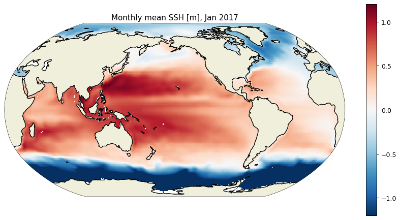
We can also use the ecco_v4_py package to plot a global map of Jan 2017 SSH, using the plot_proj_to_latlon_grid function which regrids from the native LLC grid to a lat/lon grid.

plt.figure(figsize=(12,6), dpi= 90)
ecco.plot_proj_to_latlon_grid(ds_SSH_s3.XC, ds_SSH_s3.YC, \
                              ds_SSH_s3.SSH.isel(time=0), \
                              user_lon_0=-160,\
                              projection_type='robin',\
                              plot_type='pcolormesh', \
                              cmap='RdBu_r',\
                              dx=1,dy=1,cmin=-1.2, cmax=1.2,show_colorbar=True)
plt.title('Monthly mean SSH [m], Jan 2017')
plt.show()

What if you don’t know the ShortName already?

NASA Earthdata datasets are identified by ShortNames, but you might not know the ShortName of the variable or category of variables that you are seeking. One way to find the ShortName is to consult these ECCOv4r4 variable lists. But the “query” in ecco_access functions does not have to be a ShortName; it can also be a text string representing a variable name, or a word or phrase in the variable description.

For example, perhaps you are looking to open the dataset that has native grid monthly sea ice concentration in 2007. If the query is not identified as a ShortName, then a text search of the variable lists is conducted using query, grid, and time_res. Then of the identified matches, the user is asked to select one.

ds_seaice_conc = ea.ecco_podaac_to_xrdataset('ice',grid='native',time_res='monthly',\
                                               StartDate='2007-01',EndDate='2007-12',\
                                               mode='s3_open_fsspec',\
                                               jsons_root_dir=join('/efs_ecco','mzz-jsons'))

ShortName Options for query "ice":
                  Variable Name     Description (units)

Option 1: ECCO_L4_SSH_LLC0090GRID_MONTHLY_V4R4    *native grid,monthly means*
                  SSH               Dynamic sea surface height anomaly. Suitable for
                                    comparisons with altimetry sea surface height data
                                    products that apply the inverse barometer
                                    correction. (m)
                  SSHIBC            The inverted barometer correction to sea surface
                                    height due to atmospheric pressure loading. (m)
                  SSHNOIBC          Sea surface height anomaly without the inverted
                                    barometer correction. Suitable for comparisons
                                    with altimetry sea surface height data products
                                    that do NOT apply the inverse barometer
                                    correction. (m)
                  ETAN              Model sea level anomaly, without corrections for
                                    global mean density changes, inverted barometer
                                    effect, or volume displacement due to submerged
                                    sea-ice and snow. (m)

Option 2: ECCO_L4_STRESS_LLC0090GRID_MONTHLY_V4R4    *native grid,monthly means*
                  EXFtaux           Wind stress in the model +x direction (N/m^2)
                  EXFtauy           Wind stress in the model +y direction (N/m^2)
                  oceTAUX           Ocean surface stress in the model +x direction,
                                    due to wind and sea-ice (N/m^2)
                  oceTAUY           Ocean surface stress in the model +y direction,
                                    due to wind and sea-ice (N/m^2)

Option 3: ECCO_L4_HEAT_FLUX_LLC0090GRID_MONTHLY_V4R4    *native grid,monthly means*
                  EXFhl             Open ocean air-sea latent heat flux (W/m^2)
                  EXFhs             Open ocean air-sea sensible heat flux (W/m^2)
                  EXFlwdn           Downward longwave radiative flux (W/m^2)
                  EXFswdn           Downwelling shortwave radiative flux (W/m^2)
                  EXFqnet           Open ocean net air-sea heat flux (W/m^2)
                  oceQnet           Net heat flux into the ocean surface (W/m^2)
                  SIatmQnt          Net upward heat flux to the atmosphere (W/m^2)
                  TFLUX             Rate of change of ocean heat content per m^2
                                    accounting for mass (e.g. freshwater) fluxes
                                    (W/m^2)
                  EXFswnet          Open ocean net shortwave radiative flux (W/m^2)
                  EXFlwnet          Net open ocean longwave radiative flux (W/m^2)
                  oceQsw            Net shortwave radiative flux across the ocean
                                    surface (W/m^2)
                  SIaaflux          Conservative ocean and sea-ice advective heat flux
                                    adjustment, associated with temperature difference
                                    between sea surface temperature and sea-ice,
                                    excluding latent heat of fusion (W/m^2)

Option 4: ECCO_L4_FRESH_FLUX_LLC0090GRID_MONTHLY_V4R4    *native grid,monthly means*
                  EXFpreci          Precipitation rate (m/s)
                  EXFevap           Open ocean evaporation rate (m/s)
                  EXFroff           River runoff (m/s)
                  SIsnPrcp          Snow precipitation on sea-ice (kg/(m^2 s))
                  EXFempmr          Open ocean net surface freshwater flux from
                                    precipitation, evaporation, and runoff (m/s)
                  oceFWflx          Net freshwater flux into the ocean (kg/(m^2 s))
                  SIatmFW           Net freshwater flux into the open ocean, sea-ice,
                                    and snow (kg/(m^2 s))
                  SFLUX             Rate of change of total ocean salinity per m^2
                                    accounting for mass fluxes (g/(m^2 s))
                  SIacSubl          Freshwater flux to the atmosphere due to
                                    sublimation-deposition of snow or ice (kg/(m^2 s))
                  SIrsSubl          Residual sublimation freshwater flux (kg/(m^2 s))
                  SIfwThru          Precipitation through sea-ice (kg/(m^2 s))

Option 5: ECCO_L4_SEA_ICE_CONC_THICKNESS_LLC0090GRID_MONTHLY_V4R4    *native grid,monthly means*
                  SIarea            Sea-ice concentration (fraction between 0 and 1)
                  SIheff            Area-averaged sea-ice thickness (m)
                  SIhsnow           Area-averaged snow thickness (m)
                  sIceLoad          Average sea-ice and snow mass per unit area
                                    (kg/m^2)

Option 6: ECCO_L4_SEA_ICE_VELOCITY_LLC0090GRID_MONTHLY_V4R4    *native grid,monthly means*
                  SIuice            Sea-ice velocity in the model +x direction (m/s)
                  SIvice            Sea-ice velocity in the model +y direction (m/s)

Option 7: ECCO_L4_SEA_ICE_HORIZ_VOLUME_FLUX_LLC0090GRID_MONTHLY_V4R4    *native grid,monthly means*
                  ADVxHEFF          Lateral advective flux of sea-ice thickness in the
                                    model +x direction (m^3/s)
                  ADVyHEFF          Lateral advective flux of sea-ice thickness in the
                                    model +y direction (m^3/s)
                  DFxEHEFF          Lateral diffusive flux of sea-ice thickness in the
                                    model +x direction (m^3/s)
                  DFyEHEFF          Lateral diffusive flux of sea-ice thickness in the
                                    model +y direction (m^3/s)
                  ADVxSNOW          Lateral advective flux of snow thickness in the
                                    model +x direction (m^3/s)
                  ADVySNOW          Lateral advective flux of snow thickness in the
                                    model +y direction (m^3/s)
                  DFxESNOW          Lateral diffusive flux of snow thickness in the
                                    model +x direction (m^3/s)
                  DFyESNOW          Lateral diffusive flux of snow thickness in the
                                    model +y direction (m^3/s)

Option 8: ECCO_L4_SEA_ICE_SALT_PLUME_FLUX_LLC0090GRID_MONTHLY_V4R4    *native grid,monthly means*
                  oceSPflx          Net salt flux into the ocean due to brine
                                    rejection (g/(m^2 s))
                  oceSPDep          Salt plume depth (m)


Using dataset with ShortName: ECCO_L4_SEA_ICE_CONC_THICKNESS_LLC0090GRID_MONTHLY_V4R4

We select option 5, corresponding to ShortName ECCO_L4_SEA_ICE_CONC_THICKNESS_LLC0090GRID_MONTHLY_V4R4. Let’s look at the dataset contents.

ds_seaice_conc

<xarray.Dataset> Size: 25MB
Dimensions:    (time: 12, tile: 13, j: 90, i: 90, nb: 4, j_g: 90, i_g: 90, nv: 2)
Coordinates: (12/13)
  * time       (time) datetime64[ns] 96B 2007-01-16T12:00:00 ... 2007-12-16T1...
    XC         (tile, j, i) float32 421kB dask.array<chunksize=(13, 90, 90), meta=np.ndarray>
    XC_bnds    (tile, j, i, nb) float32 2MB dask.array<chunksize=(13, 90, 90, 4), meta=np.ndarray>
    XG         (tile, j_g, i_g) float32 421kB dask.array<chunksize=(13, 90, 90), meta=np.ndarray>
    YC         (tile, j, i) float32 421kB dask.array<chunksize=(13, 90, 90), meta=np.ndarray>
    YC_bnds    (tile, j, i, nb) float32 2MB dask.array<chunksize=(13, 90, 90, 4), meta=np.ndarray>
    ...         ...
  * i          (i) int32 360B 0 1 2 3 4 5 6 7 8 9 ... 81 82 83 84 85 86 87 88 89
  * i_g        (i_g) int32 360B 0 1 2 3 4 5 6 7 8 ... 81 82 83 84 85 86 87 88 89
  * j          (j) int32 360B 0 1 2 3 4 5 6 7 8 9 ... 81 82 83 84 85 86 87 88 89
  * j_g        (j_g) int32 360B 0 1 2 3 4 5 6 7 8 ... 81 82 83 84 85 86 87 88 89
  * tile       (tile) int32 52B 0 1 2 3 4 5 6 7 8 9 10 11 12
    time_bnds  (time, nv) datetime64[ns] 192B dask.array<chunksize=(12, 2), meta=np.ndarray>
Dimensions without coordinates: nb, nv
Data variables:
    SIarea     (time, tile, j, i) float32 5MB dask.array<chunksize=(4, 13, 90, 90), meta=np.ndarray>
    SIheff     (time, tile, j, i) float32 5MB dask.array<chunksize=(4, 13, 90, 90), meta=np.ndarray>
    SIhsnow    (time, tile, j, i) float32 5MB dask.array<chunksize=(4, 13, 90, 90), meta=np.ndarray>
    sIceLoad   (time, tile, j, i) float32 5MB dask.array<chunksize=(4, 13, 90, 90), meta=np.ndarray>
Attributes: (12/57)
    Conventions:                  CF-1.8, ACDD-1.3
    acknowledgement:              This research was carried out by the Jet Pr...
    author:                       Ian Fenty and Ou Wang
    cdm_data_type:                Grid
    comment:                      Fields provided on the curvilinear lat-lon-...
    coordinates_comment:          Note: the global 'coordinates' attribute de...
    ...                           ...
    time_coverage_duration:       P1M
    time_coverage_end:            1992-02-01T00:00:00
    time_coverage_resolution:     P1M
    time_coverage_start:          1992-01-01T12:00:00
    title:                        ECCO Sea-Ice and Snow Concentration and Thi...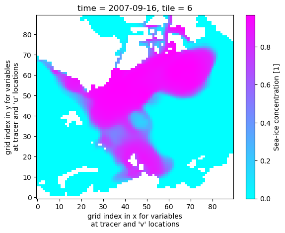
    uuid:                         cc62f1c2-400d-11eb-9f11-0cc47a3f49c3

xarray.Dataset

• Dimensions:
  • time: 12
  • tile: 13
  • j: 90
  • i: 90
  • nb: 4
  • j_g: 90
  • i_g: 90
  • nv: 2
• Coordinates: (13)
  • time
    (time)
    datetime64[ns]
    2007-01-16T12:00:00 ... 2007-12-...

    axis :

    T

    bounds :

    time_bnds

    coverage_content_type :

    coordinate

    long_name :

    center time of averaging period

    standard_name :

    time

    array(['2007-01-16T12:00:00.000000000', '2007-02-15T00:00:00.000000000',
           '2007-03-16T12:00:00.000000000', '2007-04-16T00:00:00.000000000',
           '2007-05-16T12:00:00.000000000', '2007-06-16T00:00:00.000000000',
           '2007-07-16T12:00:00.000000000', '2007-08-16T12:00:00.000000000',
           '2007-09-16T00:00:00.000000000', '2007-10-16T12:00:00.000000000',
           '2007-11-16T00:00:00.000000000', '2007-12-16T12:00:00.000000000'],
          dtype='datetime64[ns]')

  • XC
    (tile, j, i)
    float32
    dask.array<chunksize=(13, 90, 90), meta=np.ndarray>

    bounds :

    XC_bnds

    comment :

    nonuniform grid spacing

    coordinate :

    YC XC

    coverage_content_type :

    coordinate

    long_name :

    longitude of tracer grid cell center

    standard_name :

    longitude

    units :

    degrees_east

    Array Chunk Bytes 411.33 kiB 411.33 kiB Shape (13, 90, 90) (13, 90, 90) Dask graph 1 chunks in 2 graph layers Data type float32 numpy.ndarray

  • XC_bnds
    (tile, j, i, nb)
    float32
    dask.array<chunksize=(13, 90, 90, 4), meta=np.ndarray>

    comment :

    Bounds array follows CF conventions. XC_bnds[i,j,0] = 'southwest' corner (j-1, i-1), XC_bnds[i,j,1] = 'southeast' corner (j-1, i+1), XC_bnds[i,j,2] = 'northeast' corner (j+1, i+1), XC_bnds[i,j,3] = 'northwest' corner (j+1, i-1). Note: 'southwest', 'southeast', northwest', and 'northeast' do not correspond to geographic orientation but are used for convenience to describe the computational grid. See MITgcm dcoumentation for details.

    coverage_content_type :

    coordinate

    long_name :

    longitudes of tracer grid cell corners

    Array Chunk Bytes 1.61 MiB 1.61 MiB Shape (13, 90, 90, 4) (13, 90, 90, 4) Dask graph 1 chunks in 2 graph layers Data type float32 numpy.ndarray

  • XG
    (tile, j_g, i_g)
    float32
    dask.array<chunksize=(13, 90, 90), meta=np.ndarray>

    comment :

    Nonuniform grid spacing. Note: 'southwest' does not correspond to geographic orientation but is used for convenience to describe the computational grid. See MITgcm dcoumentation for details.

    coordinate :

    YG XG

    coverage_content_type :

    coordinate

    long_name :

    longitude of 'southwest' corner of tracer grid cell

    standard_name :

    longitude

    units :

    degrees_east

    Array Chunk Bytes 411.33 kiB 411.33 kiB Shape (13, 90, 90) (13, 90, 90) Dask graph 1 chunks in 2 graph layers Data type float32 numpy.ndarray

  • YC
    (tile, j, i)
    float32
    dask.array<chunksize=(13, 90, 90), meta=np.ndarray>

    bounds :

    YC_bnds

    comment :

    nonuniform grid spacing

    coordinate :

    YC XC

    coverage_content_type :

    coordinate

    long_name :

    latitude of tracer grid cell center

    standard_name :

    latitude

    units :

    degrees_north

    Array Chunk Bytes 411.33 kiB 411.33 kiB Shape (13, 90, 90) (13, 90, 90) Dask graph 1 chunks in 2 graph layers Data type float32 numpy.ndarray

  • YC_bnds
    (tile, j, i, nb)
    float32
    dask.array<chunksize=(13, 90, 90, 4), meta=np.ndarray>

    comment :

    Bounds array follows CF conventions. YC_bnds[i,j,0] = 'southwest' corner (j-1, i-1), YC_bnds[i,j,1] = 'southeast' corner (j-1, i+1), YC_bnds[i,j,2] = 'northeast' corner (j+1, i+1), YC_bnds[i,j,3] = 'northwest' corner (j+1, i-1). Note: 'southwest', 'southeast', northwest', and 'northeast' do not correspond to geographic orientation but are used for convenience to describe the computational grid. See MITgcm dcoumentation for details.

    coverage_content_type :

    coordinate

    long_name :

    latitudes of tracer grid cell corners

    Array Chunk Bytes 1.61 MiB 1.61 MiB Shape (13, 90, 90, 4) (13, 90, 90, 4) Dask graph 1 chunks in 2 graph layers Data type float32 numpy.ndarray

  • YG
    (tile, j_g, i_g)
    float32
    dask.array<chunksize=(13, 90, 90), meta=np.ndarray>

    comment :

    Nonuniform grid spacing. Note: 'southwest' does not correspond to geographic orientation but is used for convenience to describe the computational grid. See MITgcm dcoumentation for details.

    coordinate :

    YG XG

    coverage_content_type :

    coordinate

    long_name :

    latitude of 'southwest' corner of tracer grid cell

    standard_name :

    latitude

    units :

    degrees_north

    Array Chunk Bytes 411.33 kiB 411.33 kiB Shape (13, 90, 90) (13, 90, 90) Dask graph 1 chunks in 2 graph layers Data type float32 numpy.ndarray

  • i
    (i)
    int32
    0 1 2 3 4 5 6 ... 84 85 86 87 88 89

    axis :

    X

    comment :

    In the Arakawa C-grid system, tracer (e.g., THETA) and 'v' variables (e.g., VVEL) have the same x coordinate on the model grid.

    coverage_content_type :

    coordinate

    long_name :

    grid index in x for variables at tracer and 'v' locations

    swap_dim :

    XC

    array([ 0,  1,  2,  3,  4,  5,  6,  7,  8,  9, 10, 11, 12, 13, 14, 15, 16, 17,
           18, 19, 20, 21, 22, 23, 24, 25, 26, 27, 28, 29, 30, 31, 32, 33, 34, 35,
           36, 37, 38, 39, 40, 41, 42, 43, 44, 45, 46, 47, 48, 49, 50, 51, 52, 53,
           54, 55, 56, 57, 58, 59, 60, 61, 62, 63, 64, 65, 66, 67, 68, 69, 70, 71,
           72, 73, 74, 75, 76, 77, 78, 79, 80, 81, 82, 83, 84, 85, 86, 87, 88, 89],
          dtype=int32)

  • i_g
    (i_g)
    int32
    0 1 2 3 4 5 6 ... 84 85 86 87 88 89

    axis :

    X

    c_grid_axis_shift :

    -0.5

    comment :

    In the Arakawa C-grid system, 'u' (e.g., UVEL) and 'g' variables (e.g., XG) have the same x coordinate on the model grid.

    coverage_content_type :

    coordinate

    long_name :

    grid index in x for variables at 'u' and 'g' locations

    swap_dim :

    XG

    array([ 0,  1,  2,  3,  4,  5,  6,  7,  8,  9, 10, 11, 12, 13, 14, 15, 16, 17,
           18, 19, 20, 21, 22, 23, 24, 25, 26, 27, 28, 29, 30, 31, 32, 33, 34, 35,
           36, 37, 38, 39, 40, 41, 42, 43, 44, 45, 46, 47, 48, 49, 50, 51, 52, 53,
           54, 55, 56, 57, 58, 59, 60, 61, 62, 63, 64, 65, 66, 67, 68, 69, 70, 71,
           72, 73, 74, 75, 76, 77, 78, 79, 80, 81, 82, 83, 84, 85, 86, 87, 88, 89],
          dtype=int32)

  • j
    (j)
    int32
    0 1 2 3 4 5 6 ... 84 85 86 87 88 89

    axis :

    Y

    comment :

    In the Arakawa C-grid system, tracer (e.g., THETA) and 'u' variables (e.g., UVEL) have the same y coordinate on the model grid.

    coverage_content_type :

    coordinate

    long_name :

    grid index in y for variables at tracer and 'u' locations

    swap_dim :

    YC

    array([ 0,  1,  2,  3,  4,  5,  6,  7,  8,  9, 10, 11, 12, 13, 14, 15, 16, 17,
           18, 19, 20, 21, 22, 23, 24, 25, 26, 27, 28, 29, 30, 31, 32, 33, 34, 35,
           36, 37, 38, 39, 40, 41, 42, 43, 44, 45, 46, 47, 48, 49, 50, 51, 52, 53,
           54, 55, 56, 57, 58, 59, 60, 61, 62, 63, 64, 65, 66, 67, 68, 69, 70, 71,
           72, 73, 74, 75, 76, 77, 78, 79, 80, 81, 82, 83, 84, 85, 86, 87, 88, 89],
          dtype=int32)

  • j_g
    (j_g)
    int32
    0 1 2 3 4 5 6 ... 84 85 86 87 88 89

    axis :

    Y

    c_grid_axis_shift :

    -0.5

    comment :

    In the Arakawa C-grid system, 'v' (e.g., VVEL) and 'g' variables (e.g., XG) have the same y coordinate.

    coverage_content_type :

    coordinate

    long_name :

    grid index in y for variables at 'v' and 'g' locations

    swap_dim :

    YG

    array([ 0,  1,  2,  3,  4,  5,  6,  7,  8,  9, 10, 11, 12, 13, 14, 15, 16, 17,
           18, 19, 20, 21, 22, 23, 24, 25, 26, 27, 28, 29, 30, 31, 32, 33, 34, 35,
           36, 37, 38, 39, 40, 41, 42, 43, 44, 45, 46, 47, 48, 49, 50, 51, 52, 53,
           54, 55, 56, 57, 58, 59, 60, 61, 62, 63, 64, 65, 66, 67, 68, 69, 70, 71,
           72, 73, 74, 75, 76, 77, 78, 79, 80, 81, 82, 83, 84, 85, 86, 87, 88, 89],
          dtype=int32)

  • tile
    (tile)
    int32
    0 1 2 3 4 5 6 7 8 9 10 11 12

    comment :

    The ECCO V4 horizontal model grid is divided into 13 tiles of 90x90 cells for convenience.

    coverage_content_type :

    coordinate

    long_name :

    lat-lon-cap tile index

    array([ 0,  1,  2,  3,  4,  5,  6,  7,  8,  9, 10, 11, 12], dtype=int32)

  • time_bnds
    (time, nv)
    datetime64[ns]
    dask.array<chunksize=(12, 2), meta=np.ndarray>

    comment :

    Start and end times of averaging period.

    coverage_content_type :

    coordinate

    long_name :

    time bounds of averaging period

    Array Chunk Bytes 192 B 192 B Shape (12, 2) (12, 2) Dask graph 1 chunks in 3 graph layers Data type datetime64[ns] numpy.ndarray

• Data variables: (4)
  • SIarea
    (time, tile, j, i)
    float32
    dask.array<chunksize=(4, 13, 90, 90), meta=np.ndarray>

    comment :

    Fraction of ocean grid cell covered with sea-ice [0 to 1]. CF Standard Name Table v73: 'Area fraction' is the fraction of a grid cell's horizontal area that has some characteristic of interest. It is evaluated as the area of interest divided by the grid cell area. It may be expressed as a fraction, a percentage, or any other dimensionless representation of a fraction. Sea ice area fraction is area of the sea surface occupied by sea ice. It is also called 'sea ice concentration'. 'Sea ice' means all ice floating in the sea which has formed from freezing sea water, rather than by other processes such as calving of land ice to form icebergs. https://cfconventions.org/Data/cf-standard-names/73/build/cf-standard-name-table.html. Defined using CF Standard Name Table v73: 'Area fraction' is the fraction of a grid cell's horizontal area that has some characteristic of interest. It is evaluated as the area of interest divided by the grid cell area. It may be expressed as a fraction, a percentage, or any other dimensionless representation of a fraction. Sea ice area fraction is area of the sea surface occupied by sea ice. It is also called 'sea ice concentration'. 'Sea ice' means all ice floating in the sea which has formed from freezing sea water and precipitation, rather than by other processes such as calving of land ice to form icebergs. https://cfconventions.org/Data/cf-standard-names/73/build/cf-standard-name-table.html

    coverage_content_type :

    modelResult

    long_name :

    Sea-ice concentration

    standard_name :

    sea_ice_area_fraction

    units :

    1

    valid_max :

    0.9700000286102295

    valid_min :

    0.0

    Array Chunk Bytes 4.82 MiB 1.61 MiB Shape (12, 13, 90, 90) (4, 13, 90, 90) Dask graph 3 chunks in 3 graph layers Data type float32 numpy.ndarray

  • SIheff
    (time, tile, j, i)
    float32
    dask.array<chunksize=(4, 13, 90, 90), meta=np.ndarray>

    comment :

    Sea-ice thickness averaged over the entire model grid cell, including open water where sea-ice thickness is zero. Note: sea-ice thickness over the ICE-COVERED fraction of the grid cell is SIheff/SIarea

    coverage_content_type :

    modelResult

    long_name :

    Area-averaged sea-ice thickness

    standard_name :

    sea_ice_thickness

    units :

    m

    valid_max :

    7.816245079040527

    valid_min :

    0.0

    Array Chunk Bytes 4.82 MiB 1.61 MiB Shape (12, 13, 90, 90) (4, 13, 90, 90) Dask graph 3 chunks in 3 graph layers Data type float32 numpy.ndarray

  • SIhsnow
    (time, tile, j, i)
    float32
    dask.array<chunksize=(4, 13, 90, 90), meta=np.ndarray>

    comment :

    Snow thickness averaged over the entire model grid cell, including open water where snow thickness is zero. Note: snow thickness over the ICE-COVERED fraction of the grid cell is SIhsnow/SIarea

    coverage_content_type :

    modelResult

    long_name :

    Area-averaged snow thickness

    standard_name :

    surface_snow_thickness

    units :

    m

    valid_max :

    2.2215447425842285

    valid_min :

    -0.00038744235644117

    Array Chunk Bytes 4.82 MiB 1.61 MiB Shape (12, 13, 90, 90) (4, 13, 90, 90) Dask graph 3 chunks in 3 graph layers Data type float32 numpy.ndarray

  • sIceLoad
    (time, tile, j, i)
    float32
    dask.array<chunksize=(4, 13, 90, 90), meta=np.ndarray>

    comment :

    Total mass of sea-ice and snow in a model grid cell averaged over model grid cell area. Note: sIceLoad is used to correct model sea level anomaly, ETAN, to calculate dynamic sea surface height, SSH, and sea surface height without the inverted barometer (IB correction), SSHNOIBC. In the model, sea-ice is treated as floating above the sea level with ETAN tracing the location of the ocean-ice interface. Consequently, sea-ice growth in the model lowers ETAN and sea-ice melting raises ETAN. Dynamic sea surface height is obtained by correcting ETAN by the weight of ice and snow directly above following Archimedes’ principle.

    coverage_content_type :

    modelResult

    long_name :

    Average sea-ice and snow mass per unit area

    standard_name :

    sea_ice_and_surface_snow_amount

    units :

    kg m-2

    valid_max :

    7323.06005859375

    valid_min :

    -0.00011736128362827003

    Array Chunk Bytes 4.82 MiB 1.61 MiB Shape (12, 13, 90, 90) (4, 13, 90, 90) Dask graph 3 chunks in 3 graph layers Data type float32 numpy.ndarray

• Indexes: (6)
  • time
    PandasIndex

    PandasIndex(DatetimeIndex(['2007-01-16 12:00:00', '2007-02-15 00:00:00',
                   '2007-03-16 12:00:00', '2007-04-16 00:00:00',
                   '2007-05-16 12:00:00', '2007-06-16 00:00:00',
                   '2007-07-16 12:00:00', '2007-08-16 12:00:00',
                   '2007-09-16 00:00:00', '2007-10-16 12:00:00',
                   '2007-11-16 00:00:00', '2007-12-16 12:00:00'],
                  dtype='datetime64[ns]', name='time', freq=None))

  • i
    PandasIndex

    PandasIndex(Index([ 0,  1,  2,  3,  4,  5,  6,  7,  8,  9, 10, 11, 12, 13, 14, 15, 16, 17,
           18, 19, 20, 21, 22, 23, 24, 25, 26, 27, 28, 29, 30, 31, 32, 33, 34, 35,
           36, 37, 38, 39, 40, 41, 42, 43, 44, 45, 46, 47, 48, 49, 50, 51, 52, 53,
           54, 55, 56, 57, 58, 59, 60, 61, 62, 63, 64, 65, 66, 67, 68, 69, 70, 71,
           72, 73, 74, 75, 76, 77, 78, 79, 80, 81, 82, 83, 84, 85, 86, 87, 88, 89],
          dtype='int32', name='i'))

  • i_g
    PandasIndex

    PandasIndex(Index([ 0,  1,  2,  3,  4,  5,  6,  7,  8,  9, 10, 11, 12, 13, 14, 15, 16, 17,
           18, 19, 20, 21, 22, 23, 24, 25, 26, 27, 28, 29, 30, 31, 32, 33, 34, 35,
           36, 37, 38, 39, 40, 41, 42, 43, 44, 45, 46, 47, 48, 49, 50, 51, 52, 53,
           54, 55, 56, 57, 58, 59, 60, 61, 62, 63, 64, 65, 66, 67, 68, 69, 70, 71,
           72, 73, 74, 75, 76, 77, 78, 79, 80, 81, 82, 83, 84, 85, 86, 87, 88, 89],
          dtype='int32', name='i_g'))

  • j
    PandasIndex

    PandasIndex(Index([ 0,  1,  2,  3,  4,  5,  6,  7,  8,  9, 10, 11, 12, 13, 14, 15, 16, 17,
           18, 19, 20, 21, 22, 23, 24, 25, 26, 27, 28, 29, 30, 31, 32, 33, 34, 35,
           36, 37, 38, 39, 40, 41, 42, 43, 44, 45, 46, 47, 48, 49, 50, 51, 52, 53,
           54, 55, 56, 57, 58, 59, 60, 61, 62, 63, 64, 65, 66, 67, 68, 69, 70, 71,
           72, 73, 74, 75, 76, 77, 78, 79, 80, 81, 82, 83, 84, 85, 86, 87, 88, 89],
          dtype='int32', name='j'))

  • j_g
    PandasIndex

    PandasIndex(Index([ 0,  1,  2,  3,  4,  5,  6,  7,  8,  9, 10, 11, 12, 13, 14, 15, 16, 17,
           18, 19, 20, 21, 22, 23, 24, 25, 26, 27, 28, 29, 30, 31, 32, 33, 34, 35,
           36, 37, 38, 39, 40, 41, 42, 43, 44, 45, 46, 47, 48, 49, 50, 51, 52, 53,
           54, 55, 56, 57, 58, 59, 60, 61, 62, 63, 64, 65, 66, 67, 68, 69, 70, 71,
           72, 73, 74, 75, 76, 77, 78, 79, 80, 81, 82, 83, 84, 85, 86, 87, 88, 89],
          dtype='int32', name='j_g'))

  • tile
    PandasIndex

    PandasIndex(Index([0, 1, 2, 3, 4, 5, 6, 7, 8, 9, 10, 11, 12], dtype='int32', name='tile'))

• Attributes: (57)

  Conventions :

  CF-1.8, ACDD-1.3

  acknowledgement :

  This research was carried out by the Jet Propulsion Laboratory, managed by the California Institute of Technology under a contract with the National Aeronautics and Space Administration.

  author :

  Ian Fenty and Ou Wang

  cdm_data_type :

  Grid

  comment :

  Fields provided on the curvilinear lat-lon-cap 90 (llc90) native grid used in the ECCO model.

  coordinates_comment :

  Note: the global 'coordinates' attribute describes auxillary coordinates.

  creator_email :

  ecco-group@mit.edu

  creator_institution :

  NASA Jet Propulsion Laboratory (JPL)

  creator_name :

  ECCO Consortium

  creator_type :

  group

  creator_url :

  https://ecco-group.org

  date_created :

  2020-12-16T18:15:57

  date_issued :

  2020-12-16T18:15:57

  date_metadata_modified :

  2021-03-15T21:53:43

  date_modified :

  2021-03-15T21:53:43

  geospatial_bounds_crs :

  EPSG:4326

  geospatial_lat_max :

  90.0

  geospatial_lat_min :

  -90.0

  geospatial_lat_resolution :

  variable

  geospatial_lat_units :

  degrees_north

  geospatial_lon_max :

  180.0

  geospatial_lon_min :

  -180.0

  geospatial_lon_resolution :

  variable

  geospatial_lon_units :

  degrees_east

  history :

  Inaugural release of an ECCO Central Estimate solution to PO.DAAC

  id :

  10.5067/ECL5M-ICO44

  institution :

  NASA Jet Propulsion Laboratory (JPL)

  instrument_vocabulary :

  GCMD instrument keywords

  keywords :

  EARTH SCIENCE > CRYOSPHERE > SEA ICE > ICE DEPTH/THICKNESS, EARTH SCIENCE > CRYOSPHERE > SEA ICE > SEA ICE CONCENTRATION, EARTH SCIENCE > CRYOSPHERE > SEA ICE > SEA ICE CONCENTRATION > ICE FRACTION, EARTH SCIENCE SERVICES > MODELS > EARTH SCIENCE REANALYSES/ASSIMILATION MODELS, EARTH SCIENCE > CRYOSPHERE > SEA ICE > SNOW DEPTH

  keywords_vocabulary :

  NASA Global Change Master Directory (GCMD) Science Keywords

  license :

  Public Domain

  metadata_link :

  https://cmr.earthdata.nasa.gov/search/collections.umm_json?ShortName=ECCO_L4_SEA_ICE_CONC_THICKNESS_LLC0090GRID_MONTHLY_V4R4

  naming_authority :

  gov.nasa.jpl

  platform :

  ERS-1/2, TOPEX/Poseidon, Geosat Follow-On (GFO), ENVISAT, Jason-1, Jason-2, CryoSat-2, SARAL/AltiKa, Jason-3, AVHRR, Aquarius, SSM/I, SSMIS, GRACE, DTU17MDT, Argo, WOCE, GO-SHIP, MEOP, Ice Tethered Profilers (ITP)

  platform_vocabulary :

  GCMD platform keywords

  processing_level :

  L4

  product_name :

  SEA_ICE_CONC_THICKNESS_mon_mean_1992-01_ECCO_V4r4_native_llc0090.nc

  product_time_coverage_end :

  2018-01-01T00:00:00

  product_time_coverage_start :

  1992-01-01T12:00:00

  product_version :

  Version 4, Release 4

  program :

  NASA Physical Oceanography, Cryosphere, Modeling, Analysis, and Prediction (MAP)

  project :

  Estimating the Circulation and Climate of the Ocean (ECCO)

  publisher_email :

  podaac@podaac.jpl.nasa.gov

  publisher_institution :

  PO.DAAC

  publisher_name :

  Physical Oceanography Distributed Active Archive Center (PO.DAAC)

  publisher_type :

  institution

  publisher_url :

  https://podaac.jpl.nasa.gov

  references :

  ECCO Consortium, Fukumori, I., Wang, O., Fenty, I., Forget, G., Heimbach, P., & Ponte, R. M. 2020. Synopsis of the ECCO Central Production Global Ocean and Sea-Ice State Estimate (Version 4 Release 4). doi:10.5281/zenodo.3765928

  source :

  The ECCO V4r4 state estimate was produced by fitting a free-running solution of the MITgcm (checkpoint 66g) to satellite and in situ observational data in a least squares sense using the adjoint method

  standard_name_vocabulary :

  NetCDF Climate and Forecast (CF) Metadata Convention

  summary :

  This dataset provides monthly-averaged sea-ice and snow concentration, thickness, and pressure loading on the lat-lon-cap 90 (llc90) native model grid from the ECCO Version 4 Release 4 (V4r4) ocean and sea-ice state estimate. Estimating the Circulation and Climate of the Ocean (ECCO) state estimates are dynamically and kinematically-consistent reconstructions of the three-dimensional, time-evolving ocean, sea-ice, and surface atmospheric states. ECCO V4r4 is a free-running solution of a global, nominally 1-degree configuration of the MIT general circulation model (MITgcm) that has been fit to observations in a least-squares sense. Observational data constraints used in V4r4 include sea surface height (SSH) from satellite altimeters [ERS-1/2, TOPEX/Poseidon, GFO, ENVISAT, Jason-1,2,3, CryoSat-2, and SARAL/AltiKa]; sea surface temperature (SST) from satellite radiometers [AVHRR], sea surface salinity (SSS) from the Aquarius satellite radiometer/scatterometer, ocean bottom pressure (OBP) from the GRACE satellite gravimeter; sea-ice concentration from satellite radiometers [SSM/I and SSMIS], and in-situ ocean temperature and salinity measured with conductivity-temperature-depth (CTD) sensors and expendable bathythermographs (XBTs) from several programs [e.g., WOCE, GO-SHIP, Argo, and others] and platforms [e.g., research vessels, gliders, moorings, ice-tethered profilers, and instrumented pinnipeds]. V4r4 covers the period 1992-01-01T12:00:00 to 2018-01-01T00:00:00.

  time_coverage_duration :

  P1M

  time_coverage_end :

  1992-02-01T00:00:00

  time_coverage_resolution :

  P1M

  time_coverage_start :

  1992-01-01T12:00:00

  title :

  ECCO Sea-Ice and Snow Concentration and Thickness - Monthly Mean llc90 Grid (Version 4 Release 4)

  uuid :

  cc62f1c2-400d-11eb-9f11-0cc47a3f49c3

Now plot the sea ice concentration/fraction in tile 6 (which approximately covers the Arctic Ocean), during Sep 2007 which at the time was a record minimum for Arctic sea ice.

ds_seaice_conc.SIarea.isel(time=8,tile=6).plot(cmap='cool')

<matplotlib.collections.QuadMesh at 0x7ff86693d8b0>

Using the ecco_podaac_access function

In-cloud direct access (mode = ‘s3_open’)

The ecco_podaac_to_xrdataset function that was previously used invokes ecco_podaac_access under the hood, and ecco_podaac_access can also be called directly. This can be useful if you want to obtain a list of file objects/paths or URLs that you can then process with your own code. Let’s use this function with mode = s3_open (all s3 modes only work from an AWS cloud environment in region us-west-2).

curr_shortname = 'ECCO_L4_SSH_LLC0090GRID_MONTHLY_V4R4'
files_dict = ea.ecco_podaac_access(curr_shortname,\
                                    StartDate='2015-01',EndDate='2015-12',\
                                    mode='s3_open')

{'ShortName': 'ECCO_L4_SSH_LLC0090GRID_MONTHLY_V4R4', 'temporal': '2015-01-02,2015-12-31'}

Total number of matching granules: 12

files_dict[curr_shortname]

[<File-like object S3FileSystem, podaac-ops-cumulus-protected/ECCO_L4_SSH_LLC0090GRID_MONTHLY_V4R4/SEA_SURFACE_HEIGHT_mon_mean_2015-01_ECCO_V4r4_native_llc0090.nc>,
 <File-like object S3FileSystem, podaac-ops-cumulus-protected/ECCO_L4_SSH_LLC0090GRID_MONTHLY_V4R4/SEA_SURFACE_HEIGHT_mon_mean_2015-02_ECCO_V4r4_native_llc0090.nc>,
 <File-like object S3FileSystem, podaac-ops-cumulus-protected/ECCO_L4_SSH_LLC0090GRID_MONTHLY_V4R4/SEA_SURFACE_HEIGHT_mon_mean_2015-03_ECCO_V4r4_native_llc0090.nc>,
 <File-like object S3FileSystem, podaac-ops-cumulus-protected/ECCO_L4_SSH_LLC0090GRID_MONTHLY_V4R4/SEA_SURFACE_HEIGHT_mon_mean_2015-04_ECCO_V4r4_native_llc0090.nc>,
 <File-like object S3FileSystem, podaac-ops-cumulus-protected/ECCO_L4_SSH_LLC0090GRID_MONTHLY_V4R4/SEA_SURFACE_HEIGHT_mon_mean_2015-05_ECCO_V4r4_native_llc0090.nc>,
 <File-like object S3FileSystem, podaac-ops-cumulus-protected/ECCO_L4_SSH_LLC0090GRID_MONTHLY_V4R4/SEA_SURFACE_HEIGHT_mon_mean_2015-06_ECCO_V4r4_native_llc0090.nc>,
 <File-like object S3FileSystem, podaac-ops-cumulus-protected/ECCO_L4_SSH_LLC0090GRID_MONTHLY_V4R4/SEA_SURFACE_HEIGHT_mon_mean_2015-07_ECCO_V4r4_native_llc0090.nc>,
 <File-like object S3FileSystem, podaac-ops-cumulus-protected/ECCO_L4_SSH_LLC0090GRID_MONTHLY_V4R4/SEA_SURFACE_HEIGHT_mon_mean_2015-08_ECCO_V4r4_native_llc0090.nc>,
 <File-like object S3FileSystem, podaac-ops-cumulus-protected/ECCO_L4_SSH_LLC0090GRID_MONTHLY_V4R4/SEA_SURFACE_HEIGHT_mon_mean_2015-09_ECCO_V4r4_native_llc0090.nc>,
 <File-like object S3FileSystem, podaac-ops-cumulus-protected/ECCO_L4_SSH_LLC0090GRID_MONTHLY_V4R4/SEA_SURFACE_HEIGHT_mon_mean_2015-10_ECCO_V4r4_native_llc0090.nc>,
 <File-like object S3FileSystem, podaac-ops-cumulus-protected/ECCO_L4_SSH_LLC0090GRID_MONTHLY_V4R4/SEA_SURFACE_HEIGHT_mon_mean_2015-11_ECCO_V4r4_native_llc0090.nc>,
 <File-like object S3FileSystem, podaac-ops-cumulus-protected/ECCO_L4_SSH_LLC0090GRID_MONTHLY_V4R4/SEA_SURFACE_HEIGHT_mon_mean_2015-12_ECCO_V4r4_native_llc0090.nc>]

The output of ecco_podaac_access is in the form of a dictionary with ShortNames as keys. In this case, the value associated with this ShortName is a list of 12 file objects. These are files on S3 (AWS’s cloud storage system) that have been opened, which is a necessary step for the files’ data to be accessed. The list of open files can be passed directly to xarray.open_mfdataset.

ds_SSH_fromlist = xr.open_mfdataset(files_dict[curr_shortname],\
                                    compat='override',data_vars='minimal',coords='minimal',\
                                    parallel=True)

ds_SSH_fromlist

<xarray.Dataset> Size: 25MB
Dimensions:    (time: 12, tile: 13, j: 90, i: 90, i_g: 90, j_g: 90, nv: 2, nb: 4)
Coordinates: (12/13)
  * i          (i) int32 360B 0 1 2 3 4 5 6 7 8 9 ... 81 82 83 84 85 86 87 88 89
  * i_g        (i_g) int32 360B 0 1 2 3 4 5 6 7 8 ... 81 82 83 84 85 86 87 88 89
  * j          (j) int32 360B 0 1 2 3 4 5 6 7 8 9 ... 81 82 83 84 85 86 87 88 89
  * j_g        (j_g) int32 360B 0 1 2 3 4 5 6 7 8 ... 81 82 83 84 85 86 87 88 89
  * tile       (tile) int32 52B 0 1 2 3 4 5 6 7 8 9 10 11 12
  * time       (time) datetime64[ns] 96B 2015-01-16T12:00:00 ... 2015-12-16T1...
    ...         ...
    YC         (tile, j, i) float32 421kB dask.array<chunksize=(13, 90, 90), meta=np.ndarray>
    XG         (tile, j_g, i_g) float32 421kB dask.array<chunksize=(13, 90, 90), meta=np.ndarray>
    YG         (tile, j_g, i_g) float32 421kB dask.array<chunksize=(13, 90, 90), meta=np.ndarray>
    time_bnds  (time, nv) datetime64[ns] 192B dask.array<chunksize=(1, 2), meta=np.ndarray>
    XC_bnds    (tile, j, i, nb) float32 2MB dask.array<chunksize=(13, 90, 90, 4), meta=np.ndarray>
    YC_bnds    (tile, j, i, nb) float32 2MB dask.array<chunksize=(13, 90, 90, 4), meta=np.ndarray>
Dimensions without coordinates: nv, nb
Data variables:
    SSH        (time, tile, j, i) float32 5MB dask.array<chunksize=(1, 13, 90, 90), meta=np.ndarray>
    SSHIBC     (time, tile, j, i) float32 5MB dask.array<chunksize=(1, 13, 90, 90), meta=np.ndarray>
    SSHNOIBC   (time, tile, j, i) float32 5MB dask.array<chunksize=(1, 13, 90, 90), meta=np.ndarray>
    ETAN       (time, tile, j, i) float32 5MB dask.array<chunksize=(1, 13, 90, 90), meta=np.ndarray>
Attributes: (12/57)
    acknowledgement:              This research was carried out by the Jet Pr...
    author:                       Ian Fenty and Ou Wang
    cdm_data_type:                Grid
    comment:                      Fields provided on the curvilinear lat-lon-...
    Conventions:                  CF-1.8, ACDD-1.3
    coordinates_comment:          Note: the global 'coordinates' attribute de...
    ...                           ...
    time_coverage_duration:       P1M
    time_coverage_end:            2015-02-01T00:00:00
    time_coverage_resolution:     P1M
    time_coverage_start:          2015-01-01T00:00:00
    title:                        ECCO Sea Surface Height - Monthly Mean llc9...
    uuid:                         a4955186-400c-11eb-8c14-0cc47a3f49c3

xarray.Dataset

• Dimensions:
  • time: 12
  • tile: 13
  • j: 90
  • i: 90
  • i_g: 90
  • j_g: 90
  • nv: 2
  • nb: 4
• Coordinates: (13)
  • i
    (i)
    int32
    0 1 2 3 4 5 6 ... 84 85 86 87 88 89

    axis :

    X

    long_name :

    grid index in x for variables at tracer and 'v' locations

    swap_dim :

    XC

    comment :

    In the Arakawa C-grid system, tracer (e.g., THETA) and 'v' variables (e.g., VVEL) have the same x coordinate on the model grid.

    coverage_content_type :

    coordinate

    array([ 0,  1,  2,  3,  4,  5,  6,  7,  8,  9, 10, 11, 12, 13, 14, 15, 16, 17,
           18, 19, 20, 21, 22, 23, 24, 25, 26, 27, 28, 29, 30, 31, 32, 33, 34, 35,
           36, 37, 38, 39, 40, 41, 42, 43, 44, 45, 46, 47, 48, 49, 50, 51, 52, 53,
           54, 55, 56, 57, 58, 59, 60, 61, 62, 63, 64, 65, 66, 67, 68, 69, 70, 71,
           72, 73, 74, 75, 76, 77, 78, 79, 80, 81, 82, 83, 84, 85, 86, 87, 88, 89],
          dtype=int32)

  • i_g
    (i_g)
    int32
    0 1 2 3 4 5 6 ... 84 85 86 87 88 89

    axis :

    X

    long_name :

    grid index in x for variables at 'u' and 'g' locations

    c_grid_axis_shift :

    -0.5

    swap_dim :

    XG

    comment :

    In the Arakawa C-grid system, 'u' (e.g., UVEL) and 'g' variables (e.g., XG) have the same x coordinate on the model grid.

    coverage_content_type :

    coordinate

    array([ 0,  1,  2,  3,  4,  5,  6,  7,  8,  9, 10, 11, 12, 13, 14, 15, 16, 17,
           18, 19, 20, 21, 22, 23, 24, 25, 26, 27, 28, 29, 30, 31, 32, 33, 34, 35,
           36, 37, 38, 39, 40, 41, 42, 43, 44, 45, 46, 47, 48, 49, 50, 51, 52, 53,
           54, 55, 56, 57, 58, 59, 60, 61, 62, 63, 64, 65, 66, 67, 68, 69, 70, 71,
           72, 73, 74, 75, 76, 77, 78, 79, 80, 81, 82, 83, 84, 85, 86, 87, 88, 89],
          dtype=int32)

  • j
    (j)
    int32
    0 1 2 3 4 5 6 ... 84 85 86 87 88 89

    axis :

    Y

    long_name :

    grid index in y for variables at tracer and 'u' locations

    swap_dim :

    YC

    comment :

    In the Arakawa C-grid system, tracer (e.g., THETA) and 'u' variables (e.g., UVEL) have the same y coordinate on the model grid.

    coverage_content_type :

    coordinate

    array([ 0,  1,  2,  3,  4,  5,  6,  7,  8,  9, 10, 11, 12, 13, 14, 15, 16, 17,
           18, 19, 20, 21, 22, 23, 24, 25, 26, 27, 28, 29, 30, 31, 32, 33, 34, 35,
           36, 37, 38, 39, 40, 41, 42, 43, 44, 45, 46, 47, 48, 49, 50, 51, 52, 53,
           54, 55, 56, 57, 58, 59, 60, 61, 62, 63, 64, 65, 66, 67, 68, 69, 70, 71,
           72, 73, 74, 75, 76, 77, 78, 79, 80, 81, 82, 83, 84, 85, 86, 87, 88, 89],
          dtype=int32)

  • j_g
    (j_g)
    int32
    0 1 2 3 4 5 6 ... 84 85 86 87 88 89

    axis :

    Y

    long_name :

    grid index in y for variables at 'v' and 'g' locations

    c_grid_axis_shift :

    -0.5

    swap_dim :

    YG

    comment :

    In the Arakawa C-grid system, 'v' (e.g., VVEL) and 'g' variables (e.g., XG) have the same y coordinate.

    coverage_content_type :

    coordinate

    array([ 0,  1,  2,  3,  4,  5,  6,  7,  8,  9, 10, 11, 12, 13, 14, 15, 16, 17,
           18, 19, 20, 21, 22, 23, 24, 25, 26, 27, 28, 29, 30, 31, 32, 33, 34, 35,
           36, 37, 38, 39, 40, 41, 42, 43, 44, 45, 46, 47, 48, 49, 50, 51, 52, 53,
           54, 55, 56, 57, 58, 59, 60, 61, 62, 63, 64, 65, 66, 67, 68, 69, 70, 71,
           72, 73, 74, 75, 76, 77, 78, 79, 80, 81, 82, 83, 84, 85, 86, 87, 88, 89],
          dtype=int32)

  • tile
    (tile)
    int32
    0 1 2 3 4 5 6 7 8 9 10 11 12

    long_name :

    lat-lon-cap tile index

    comment :

    The ECCO V4 horizontal model grid is divided into 13 tiles of 90x90 cells for convenience.

    coverage_content_type :

    coordinate

    array([ 0,  1,  2,  3,  4,  5,  6,  7,  8,  9, 10, 11, 12], dtype=int32)

  • time
    (time)
    datetime64[ns]
    2015-01-16T12:00:00 ... 2015-12-...

    long_name :

    center time of averaging period

    axis :

    T

    bounds :

    time_bnds

    coverage_content_type :

    coordinate

    standard_name :

    time

    array(['2015-01-16T12:00:00.000000000', '2015-02-15T00:00:00.000000000',
           '2015-03-16T12:00:00.000000000', '2015-04-16T00:00:00.000000000',
           '2015-05-16T12:00:00.000000000', '2015-06-16T00:00:00.000000000',
           '2015-07-16T12:00:00.000000000', '2015-08-16T12:00:00.000000000',
           '2015-09-16T00:00:00.000000000', '2015-10-16T12:00:00.000000000',
           '2015-11-16T00:00:00.000000000', '2015-12-16T12:00:00.000000000'],
          dtype='datetime64[ns]')

  • XC
    (tile, j, i)
    float32
    dask.array<chunksize=(13, 90, 90), meta=np.ndarray>

    long_name :

    longitude of tracer grid cell center

    units :

    degrees_east

    coordinate :

    YC XC

    bounds :

    XC_bnds

    comment :

    nonuniform grid spacing

    coverage_content_type :

    coordinate

    standard_name :

    longitude

    Array Chunk Bytes 411.33 kiB 411.33 kiB Shape (13, 90, 90) (13, 90, 90) Dask graph 1 chunks in 2 graph layers Data type float32 numpy.ndarray

  • YC
    (tile, j, i)
    float32
    dask.array<chunksize=(13, 90, 90), meta=np.ndarray>

    long_name :

    latitude of tracer grid cell center

    units :

    degrees_north

    coordinate :

    YC XC

    bounds :

    YC_bnds

    comment :

    nonuniform grid spacing

    coverage_content_type :

    coordinate

    standard_name :

    latitude

    Array Chunk Bytes 411.33 kiB 411.33 kiB Shape (13, 90, 90) (13, 90, 90) Dask graph 1 chunks in 2 graph layers Data type float32 numpy.ndarray

  • XG
    (tile, j_g, i_g)
    float32
    dask.array<chunksize=(13, 90, 90), meta=np.ndarray>

    long_name :

    longitude of 'southwest' corner of tracer grid cell

    units :

    degrees_east

    coordinate :

    YG XG

    comment :

    Nonuniform grid spacing. Note: 'southwest' does not correspond to geographic orientation but is used for convenience to describe the computational grid. See MITgcm dcoumentation for details.

    coverage_content_type :

    coordinate

    standard_name :

    longitude

    Array Chunk Bytes 411.33 kiB 411.33 kiB Shape (13, 90, 90) (13, 90, 90) Dask graph 1 chunks in 2 graph layers Data type float32 numpy.ndarray

  • YG
    (tile, j_g, i_g)
    float32
    dask.array<chunksize=(13, 90, 90), meta=np.ndarray>

    long_name :

    latitude of 'southwest' corner of tracer grid cell

    units :

    degrees_north

    coordinate :

    YG XG

    comment :

    Nonuniform grid spacing. Note: 'southwest' does not correspond to geographic orientation but is used for convenience to describe the computational grid. See MITgcm dcoumentation for details.

    coverage_content_type :

    coordinate

    standard_name :

    latitude

    Array Chunk Bytes 411.33 kiB 411.33 kiB Shape (13, 90, 90) (13, 90, 90) Dask graph 1 chunks in 2 graph layers Data type float32 numpy.ndarray

  • time_bnds
    (time, nv)
    datetime64[ns]
    dask.array<chunksize=(1, 2), meta=np.ndarray>

    comment :

    Start and end times of averaging period.

    coverage_content_type :

    coordinate

    long_name :

    time bounds of averaging period

    Array Chunk Bytes 192 B 16 B Shape (12, 2) (1, 2) Dask graph 12 chunks in 25 graph layers Data type datetime64[ns] numpy.ndarray

  • XC_bnds
    (tile, j, i, nb)
    float32
    dask.array<chunksize=(13, 90, 90, 4), meta=np.ndarray>

    comment :

    Bounds array follows CF conventions. XC_bnds[i,j,0] = 'southwest' corner (j-1, i-1), XC_bnds[i,j,1] = 'southeast' corner (j-1, i+1), XC_bnds[i,j,2] = 'northeast' corner (j+1, i+1), XC_bnds[i,j,3] = 'northwest' corner (j+1, i-1). Note: 'southwest', 'southeast', northwest', and 'northeast' do not correspond to geographic orientation but are used for convenience to describe the computational grid. See MITgcm dcoumentation for details.

    coverage_content_type :

    coordinate

    long_name :

    longitudes of tracer grid cell corners

    Array Chunk Bytes 1.61 MiB 1.61 MiB Shape (13, 90, 90, 4) (13, 90, 90, 4) Dask graph 1 chunks in 2 graph layers Data type float32 numpy.ndarray

  • YC_bnds
    (tile, j, i, nb)
    float32
    dask.array<chunksize=(13, 90, 90, 4), meta=np.ndarray>

    comment :

    Bounds array follows CF conventions. YC_bnds[i,j,0] = 'southwest' corner (j-1, i-1), YC_bnds[i,j,1] = 'southeast' corner (j-1, i+1), YC_bnds[i,j,2] = 'northeast' corner (j+1, i+1), YC_bnds[i,j,3] = 'northwest' corner (j+1, i-1). Note: 'southwest', 'southeast', northwest', and 'northeast' do not correspond to geographic orientation but are used for convenience to describe the computational grid. See MITgcm dcoumentation for details.

    coverage_content_type :

    coordinate

    long_name :

    latitudes of tracer grid cell corners

    Array Chunk Bytes 1.61 MiB 1.61 MiB Shape (13, 90, 90, 4) (13, 90, 90, 4) Dask graph 1 chunks in 2 graph layers Data type float32 numpy.ndarray

• Data variables: (4)
  • SSH
    (time, tile, j, i)
    float32
    dask.array<chunksize=(1, 13, 90, 90), meta=np.ndarray>

    long_name :

    Dynamic sea surface height anomaly

    units :

    m

    coverage_content_type :

    modelResult

    standard_name :

    sea_surface_height_above_geoid

    comment :

    Dynamic sea surface height anomaly above the geoid, suitable for comparisons with altimetry sea surface height data products that apply the inverse barometer (IB) correction. Note: SSH is calculated by correcting model sea level anomaly ETAN for three effects: a) global mean steric sea level changes related to density changes in the Boussinesq volume-conserving model (Greatbatch correction, see sterGloH), b) the inverted barometer (IB) effect (see SSHIBC) and c) sea level displacement due to sea-ice and snow pressure loading (see sIceLoad). SSH can be compared with the similarly-named SSH variable in previous ECCO products that did not include atmospheric pressure loading (e.g., Version 4 Release 3). Use SSHNOIBC for comparisons with altimetry data products that do NOT apply the IB correction.

    valid_min :

    -1.8805772066116333

    valid_max :

    1.4207719564437866

    Array Chunk Bytes 4.82 MiB 411.33 kiB Shape (12, 13, 90, 90) (1, 13, 90, 90) Dask graph 12 chunks in 25 graph layers Data type float32 numpy.ndarray

  • SSHIBC
    (time, tile, j, i)
    float32
    dask.array<chunksize=(1, 13, 90, 90), meta=np.ndarray>

    long_name :

    The inverted barometer (IB) correction to sea surface height due to atmospheric pressure loading

    units :

    m

    coverage_content_type :

    modelResult

    comment :

    Not an SSH itself, but a correction to model sea level anomaly (ETAN) required to account for the static part of sea surface displacement by atmosphere pressure loading: SSH = SSHNOIBC - SSHIBC. Note: Use SSH for model-data comparisons with altimetry data products that DO apply the IB correction and SSHNOIBC for comparisons with altimetry data products that do NOT apply the IB correction.

    valid_min :

    -0.30144819617271423

    valid_max :

    0.5248842239379883

    Array Chunk Bytes 4.82 MiB 411.33 kiB Shape (12, 13, 90, 90) (1, 13, 90, 90) Dask graph 12 chunks in 25 graph layers Data type float32 numpy.ndarray

  • SSHNOIBC
    (time, tile, j, i)
    float32
    dask.array<chunksize=(1, 13, 90, 90), meta=np.ndarray>

    long_name :

    Sea surface height anomaly without the inverted barometer (IB) correction

    units :

    m

    coverage_content_type :

    modelResult

    comment :

    Sea surface height anomaly above the geoid without the inverse barometer (IB) correction, suitable for comparisons with altimetry sea surface height data products that do NOT apply the inverse barometer (IB) correction. Note: SSHNOIBC is calculated by correcting model sea level anomaly ETAN for two effects: a) global mean steric sea level changes related to density changes in the Boussinesq volume-conserving model (Greatbatch correction, see sterGloH), b) sea level displacement due to sea-ice and snow pressure loading (see sIceLoad). In ECCO Version 4 Release 4 the model is forced with atmospheric pressure loading. SSHNOIBC does not correct for the static part of the effect of atmosphere pressure loading on sea surface height (the so-called inverse barometer (IB) correction). Use SSH for comparisons with altimetry data products that DO apply the IB correction.

    valid_min :

    -1.6654272079467773

    valid_max :

    1.4550364017486572

    Array Chunk Bytes 4.82 MiB 411.33 kiB Shape (12, 13, 90, 90) (1, 13, 90, 90) Dask graph 12 chunks in 25 graph layers Data type float32 numpy.ndarray

  • ETAN
    (time, tile, j, i)
    float32
    dask.array<chunksize=(1, 13, 90, 90), meta=np.ndarray>

    long_name :

    Model sea level anomaly

    units :

    m

    coverage_content_type :

    modelResult

    comment :

    Model sea level anomaly WITHOUT corrections for global mean density (steric) changes, inverted barometer effect, or volume displacement due to submerged sea-ice and snow . Note: ETAN should NOT be used for comparisons with altimetry data products because ETAN is NOT corrected for (a) global mean steric sea level changes related to density changes in the Boussinesq volume-conserving model (Greatbatch correction, see sterGloH) nor (b) sea level displacement due to submerged sea-ice and snow (see sIceLoad). These corrections ARE made for the variables SSH and SSHNOIBC.

    valid_min :

    -8.304216384887695

    valid_max :

    1.460192084312439

    Array Chunk Bytes 4.82 MiB 411.33 kiB Shape (12, 13, 90, 90) (1, 13, 90, 90) Dask graph 12 chunks in 25 graph layers Data type float32 numpy.ndarray

• Indexes: (6)
  • i
    PandasIndex

    PandasIndex(Index([ 0,  1,  2,  3,  4,  5,  6,  7,  8,  9, 10, 11, 12, 13, 14, 15, 16, 17,
           18, 19, 20, 21, 22, 23, 24, 25, 26, 27, 28, 29, 30, 31, 32, 33, 34, 35,
           36, 37, 38, 39, 40, 41, 42, 43, 44, 45, 46, 47, 48, 49, 50, 51, 52, 53,
           54, 55, 56, 57, 58, 59, 60, 61, 62, 63, 64, 65, 66, 67, 68, 69, 70, 71,
           72, 73, 74, 75, 76, 77, 78, 79, 80, 81, 82, 83, 84, 85, 86, 87, 88, 89],
          dtype='int32', name='i'))

  • i_g
    PandasIndex

    PandasIndex(Index([ 0,  1,  2,  3,  4,  5,  6,  7,  8,  9, 10, 11, 12, 13, 14, 15, 16, 17,
           18, 19, 20, 21, 22, 23, 24, 25, 26, 27, 28, 29, 30, 31, 32, 33, 34, 35,
           36, 37, 38, 39, 40, 41, 42, 43, 44, 45, 46, 47, 48, 49, 50, 51, 52, 53,
           54, 55, 56, 57, 58, 59, 60, 61, 62, 63, 64, 65, 66, 67, 68, 69, 70, 71,
           72, 73, 74, 75, 76, 77, 78, 79, 80, 81, 82, 83, 84, 85, 86, 87, 88, 89],
          dtype='int32', name='i_g'))

  • j
    PandasIndex

    PandasIndex(Index([ 0,  1,  2,  3,  4,  5,  6,  7,  8,  9, 10, 11, 12, 13, 14, 15, 16, 17,
           18, 19, 20, 21, 22, 23, 24, 25, 26, 27, 28, 29, 30, 31, 32, 33, 34, 35,
           36, 37, 38, 39, 40, 41, 42, 43, 44, 45, 46, 47, 48, 49, 50, 51, 52, 53,
           54, 55, 56, 57, 58, 59, 60, 61, 62, 63, 64, 65, 66, 67, 68, 69, 70, 71,
           72, 73, 74, 75, 76, 77, 78, 79, 80, 81, 82, 83, 84, 85, 86, 87, 88, 89],
          dtype='int32', name='j'))

  • j_g
    PandasIndex

    PandasIndex(Index([ 0,  1,  2,  3,  4,  5,  6,  7,  8,  9, 10, 11, 12, 13, 14, 15, 16, 17,
           18, 19, 20, 21, 22, 23, 24, 25, 26, 27, 28, 29, 30, 31, 32, 33, 34, 35,
           36, 37, 38, 39, 40, 41, 42, 43, 44, 45, 46, 47, 48, 49, 50, 51, 52, 53,
           54, 55, 56, 57, 58, 59, 60, 61, 62, 63, 64, 65, 66, 67, 68, 69, 70, 71,
           72, 73, 74, 75, 76, 77, 78, 79, 80, 81, 82, 83, 84, 85, 86, 87, 88, 89],
          dtype='int32', name='j_g'))

  • tile
    PandasIndex

    PandasIndex(Index([0, 1, 2, 3, 4, 5, 6, 7, 8, 9, 10, 11, 12], dtype='int32', name='tile'))

  • time
    PandasIndex

    PandasIndex(DatetimeIndex(['2015-01-16 12:00:00', '2015-02-15 00:00:00',
                   '2015-03-16 12:00:00', '2015-04-16 00:00:00',
                   '2015-05-16 12:00:00', '2015-06-16 00:00:00',
                   '2015-07-16 12:00:00', '2015-08-16 12:00:00',
                   '2015-09-16 00:00:00', '2015-10-16 12:00:00',
                   '2015-11-16 00:00:00', '2015-12-16 12:00:00'],
                  dtype='datetime64[ns]', name='time', freq=None))

• Attributes: (57)

  acknowledgement :

  This research was carried out by the Jet Propulsion Laboratory, managed by the California Institute of Technology under a contract with the National Aeronautics and Space Administration.

  author :

  Ian Fenty and Ou Wang

  cdm_data_type :

  Grid

  comment :

  Fields provided on the curvilinear lat-lon-cap 90 (llc90) native grid used in the ECCO model. SSH (dynamic sea surface height) = SSHNOIBC (dynamic sea surface without the inverse barometer correction) - SSHIBC (inverse barometer correction). The inverted barometer correction accounts for variations in sea surface height due to atmospheric pressure variations. Note: ETAN is model sea level anomaly and should not be compared with satellite altimetery products, see SSH and ETAN for more details.

  Conventions :

  CF-1.8, ACDD-1.3

  coordinates_comment :

  Note: the global 'coordinates' attribute describes auxillary coordinates.

  creator_email :

  ecco-group@mit.edu

  creator_institution :

  NASA Jet Propulsion Laboratory (JPL)

  creator_name :

  ECCO Consortium

  creator_type :

  group

  creator_url :

  https://ecco-group.org

  date_created :

  2020-12-16T18:07:40

  date_issued :

  2020-12-16T18:07:40

  date_metadata_modified :

  2021-03-15T21:56:49

  date_modified :

  2021-03-15T21:56:49

  geospatial_bounds_crs :

  EPSG:4326

  geospatial_lat_max :

  90.0

  geospatial_lat_min :

  -90.0

  geospatial_lat_resolution :

  variable

  geospatial_lat_units :

  degrees_north

  geospatial_lon_max :

  180.0

  geospatial_lon_min :

  -180.0

  geospatial_lon_resolution :

  variable

  geospatial_lon_units :

  degrees_east

  history :

  Inaugural release of an ECCO Central Estimate solution to PO.DAAC

  id :

  10.5067/ECL5M-SSH44

  institution :

  NASA Jet Propulsion Laboratory (JPL)

  instrument_vocabulary :

  GCMD instrument keywords

  keywords :

  EARTH SCIENCE SERVICES > MODELS > EARTH SCIENCE REANALYSES/ASSIMILATION MODELS, EARTH SCIENCE > OCEANS > SEA SURFACE TOPOGRAPHY > SEA SURFACE HEIGHT

  keywords_vocabulary :

  NASA Global Change Master Directory (GCMD) Science Keywords

  license :

  Public Domain

  metadata_link :

  https://cmr.earthdata.nasa.gov/search/collections.umm_json?ShortName=ECCO_L4_SSH_LLC0090GRID_MONTHLY_V4R4

  naming_authority :

  gov.nasa.jpl

  platform :

  ERS-1/2, TOPEX/Poseidon, Geosat Follow-On (GFO), ENVISAT, Jason-1, Jason-2, CryoSat-2, SARAL/AltiKa, Jason-3, AVHRR, Aquarius, SSM/I, SSMIS, GRACE, DTU17MDT, Argo, WOCE, GO-SHIP, MEOP, Ice Tethered Profilers (ITP)

  platform_vocabulary :

  GCMD platform keywords

  processing_level :

  L4

  product_name :

  SEA_SURFACE_HEIGHT_mon_mean_2015-01_ECCO_V4r4_native_llc0090.nc

  product_time_coverage_end :

  2018-01-01T00:00:00

  product_time_coverage_start :

  1992-01-01T12:00:00

  product_version :

  Version 4, Release 4

  program :

  NASA Physical Oceanography, Cryosphere, Modeling, Analysis, and Prediction (MAP)

  project :

  Estimating the Circulation and Climate of the Ocean (ECCO)

  publisher_email :

  podaac@podaac.jpl.nasa.gov

  publisher_institution :

  PO.DAAC

  publisher_name :

  Physical Oceanography Distributed Active Archive Center (PO.DAAC)

  publisher_type :

  institution

  publisher_url :

  https://podaac.jpl.nasa.gov

  references :

  ECCO Consortium, Fukumori, I., Wang, O., Fenty, I., Forget, G., Heimbach, P., & Ponte, R. M. 2020. Synopsis of the ECCO Central Production Global Ocean and Sea-Ice State Estimate (Version 4 Release 4). doi:10.5281/zenodo.3765928

  source :

  The ECCO V4r4 state estimate was produced by fitting a free-running solution of the MITgcm (checkpoint 66g) to satellite and in situ observational data in a least squares sense using the adjoint method

  standard_name_vocabulary :

  NetCDF Climate and Forecast (CF) Metadata Convention

  summary :

  This dataset provides monthly-averaged dynamic sea surface height and model sea level anomaly on the lat-lon-cap 90 (llc90) native model grid from the ECCO Version 4 Release 4 (V4r4) ocean and sea-ice state estimate. Estimating the Circulation and Climate of the Ocean (ECCO) state estimates are dynamically and kinematically-consistent reconstructions of the three-dimensional, time-evolving ocean, sea-ice, and surface atmospheric states. ECCO V4r4 is a free-running solution of a global, nominally 1-degree configuration of the MIT general circulation model (MITgcm) that has been fit to observations in a least-squares sense. Observational data constraints used in V4r4 include sea surface height (SSH) from satellite altimeters [ERS-1/2, TOPEX/Poseidon, GFO, ENVISAT, Jason-1,2,3, CryoSat-2, and SARAL/AltiKa]; sea surface temperature (SST) from satellite radiometers [AVHRR], sea surface salinity (SSS) from the Aquarius satellite radiometer/scatterometer, ocean bottom pressure (OBP) from the GRACE satellite gravimeter; sea-ice concentration from satellite radiometers [SSM/I and SSMIS], and in-situ ocean temperature and salinity measured with conductivity-temperature-depth (CTD) sensors and expendable bathythermographs (XBTs) from several programs [e.g., WOCE, GO-SHIP, Argo, and others] and platforms [e.g., research vessels, gliders, moorings, ice-tethered profilers, and instrumented pinnipeds]. V4r4 covers the period 1992-01-01T12:00:00 to 2018-01-01T00:00:00.

  time_coverage_duration :

  P1M

  time_coverage_end :

  2015-02-01T00:00:00

  time_coverage_resolution :

  P1M

  time_coverage_start :

  2015-01-01T00:00:00

  title :

  ECCO Sea Surface Height - Monthly Mean llc90 Grid (Version 4 Release 4)

  uuid :

  a4955186-400c-11eb-8c14-0cc47a3f49c3

Accessing ECCOv4 release 5 output

In addition to accessing the ECCOv4r4 Central Estimate output released on PO.DAAC, ecco_access functions can also retrieve output from the newer release 5 (ECCOv4r5). Unlike v4r4, for which many fields can be accessed at monthly/daily/snapshot time resolutions and native/latlon grid configurations, only the v4r5 monthly mean native grid outputs are currently accessible, and only working within the AWS Cloud. However, a number of fields were archived in v4r5 that were not archived in v4r4, including the terms of momentum and sea-ice budgets.

Note

When accessing v4r5 output using mode = s3_open_fsspec, the jsons_root_dir on OSS/P-cluster is /efs_ecco/mzz-jsons-V4r5. If join has been imported from os.path, this can also be written as jsons_root_dir=join('/efs_ecco','mzz-jsons-V4r5').

SST comparison: v4r4 vs. v4r5

First let’s consider a field that is archived in both releases: potential temperature in the top layer, or SST. Accessing the monthly mean potential temperature for 1998 from v4r4 (and assuming we don’t know the ShortName already):

ds_T_v4r4 = ea.ecco_podaac_to_xrdataset('temperature',\
                                            version='v4r4',grid='native',time_res='monthly',\
                                            StartDate='1998-01',EndDate='1998-12',\
                                            mode='s3_open_fsspec',\
                                            jsons_root_dir=join('/efs_ecco','mzz-jsons'))

ShortName Options for query "temperature":
                  Variable Name     Description (units)

Option 1: ECCO_L4_ATM_STATE_LLC0090GRID_MONTHLY_V4R4    *native grid,monthly means*
                  EXFatemp          Atmosphere surface (2 m) air temperature (degK)
                  EXFaqh            Atmosphere surface (2 m) specific humidity (kg/kg)
                  EXFuwind          Wind speed at 10m in the model +x direction (m/s)
                  EXFvwind          Wind speed at 10m in the model +y direction (m/s)
                  EXFwspee          Wind speed (m/s)
                  EXFpress          Atmosphere surface pressure (N/m^2)

Option 2: ECCO_L4_HEAT_FLUX_LLC0090GRID_MONTHLY_V4R4    *native grid,monthly means*
                  EXFhl             Open ocean air-sea latent heat flux (W/m^2)
                  EXFhs             Open ocean air-sea sensible heat flux (W/m^2)
                  EXFlwdn           Downward longwave radiative flux (W/m^2)
                  EXFswdn           Downwelling shortwave radiative flux (W/m^2)
                  EXFqnet           Open ocean net air-sea heat flux (W/m^2)
                  oceQnet           Net heat flux into the ocean surface (W/m^2)
                  SIatmQnt          Net upward heat flux to the atmosphere (W/m^2)
                  TFLUX             Rate of change of ocean heat content per m^2
                                    accounting for mass (e.g. freshwater) fluxes
                                    (W/m^2)
                  EXFswnet          Open ocean net shortwave radiative flux (W/m^2)
                  EXFlwnet          Net open ocean longwave radiative flux (W/m^2)
                  oceQsw            Net shortwave radiative flux across the ocean
                                    surface (W/m^2)
                  SIaaflux          Conservative ocean and sea-ice advective heat flux
                                    adjustment, associated with temperature difference
                                    between sea surface temperature and sea-ice,
                                    excluding latent heat of fusion (W/m^2)

Option 3: ECCO_L4_MIXED_LAYER_DEPTH_LLC0090GRID_MONTHLY_V4R4    *native grid,monthly means*
                  MXLDEPTH          Mixed-layer depth diagnosed using the temperature
                                    difference criterion of Kara et al., 2000 (m)

Option 4: ECCO_L4_TEMP_SALINITY_LLC0090GRID_MONTHLY_V4R4    *native grid,monthly means*
                  THETA             Potential temperature, i.e., temperature of water
                                    parcel at sea level pressure (degC)
                  SALT              Salinity (1e-3, or parts per thousand)

Option 5: ECCO_L4_OCEAN_3D_TEMPERATURE_FLUX_LLC0090GRID_MONTHLY_V4R4    *native grid,monthly means*
                  ADVx_TH           Lateral advective flux of potential temperature in
                                    the model +x direction (degC m^3/s)
                  ADVy_TH           Lateral advective flux of potential temperature in
                                    the model +y direction (degC m^3/s)
                  ADVr_TH           Vertical advective flux of potential temperature
                                    (degC m^3/s)
                  DFxE_TH           Lateral diffusive flux of potential temperature in
                                    the model +x direction (degC m^3/s)
                  DFyE_TH           Lateral diffusive flux of potential temperature in
                                    the model +y direction (degC m^3/s)
                  DFrE_TH           Vertical diffusive flux of potential temperature,
                                    explicit term (degC m^3/s)
                  DFrI_TH           Vertical diffusive flux of potential temperature,
                                    implicit term (degC m^3/s)


Using dataset with ShortName: ECCO_L4_TEMP_SALINITY_LLC0090GRID_MONTHLY_V4R4

Select option 4 (the dataset that contains variables THETA and SALT), and the requested output is included in the xarray dataset ds_T_v4r4. Here is the contents of that dataset:

ds_T_v4r4

<xarray.Dataset> Size: 510MB
Dimensions:    (time: 12, k: 50, tile: 13, j: 90, i: 90, nb: 4, j_g: 90,
                i_g: 90, nv: 2, k_l: 50, k_p1: 51, k_u: 50)
Coordinates: (12/22)
  * time       (time) datetime64[ns] 96B 1998-01-16T12:00:00 ... 1998-12-16T1...
    XC         (tile, j, i) float32 421kB dask.array<chunksize=(13, 90, 90), meta=np.ndarray>
    XC_bnds    (tile, j, i, nb) float32 2MB dask.array<chunksize=(13, 90, 90, 4), meta=np.ndarray>
    XG         (tile, j_g, i_g) float32 421kB dask.array<chunksize=(13, 90, 90), meta=np.ndarray>
    YC         (tile, j, i) float32 421kB dask.array<chunksize=(13, 90, 90), meta=np.ndarray>
    YC_bnds    (tile, j, i, nb) float32 2MB dask.array<chunksize=(13, 90, 90, 4), meta=np.ndarray>
    ...         ...
  * k          (k) int32 200B 0 1 2 3 4 5 6 7 8 9 ... 41 42 43 44 45 46 47 48 49
  * k_l        (k_l) int32 200B 0 1 2 3 4 5 6 7 8 ... 41 42 43 44 45 46 47 48 49
  * k_p1       (k_p1) int32 204B 0 1 2 3 4 5 6 7 8 ... 43 44 45 46 47 48 49 50
  * k_u        (k_u) int32 200B 0 1 2 3 4 5 6 7 8 ... 41 42 43 44 45 46 47 48 49
  * tile       (tile) int32 52B 0 1 2 3 4 5 6 7 8 9 10 11 12
    time_bnds  (time, nv) datetime64[ns] 192B dask.array<chunksize=(12, 2), meta=np.ndarray>
Dimensions without coordinates: nb, nv
Data variables:
    SALT       (time, k, tile, j, i) float32 253MB dask.array<chunksize=(6, 50, 13, 90, 90), meta=np.ndarray>
    THETA      (time, k, tile, j, i) float32 253MB dask.array<chunksize=(6, 50, 13, 90, 90), meta=np.ndarray>
Attributes: (12/62)
    Conventions:                     CF-1.8, ACDD-1.3
    acknowledgement:                 This research was carried out by the Jet...
    author:                          Ian Fenty and Ou Wang
    cdm_data_type:                   Grid
    comment:                         Fields provided on the curvilinear lat-l...
    coordinates_comment:             Note: the global 'coordinates' attribute...
    ...                              ...
    time_coverage_duration:          P1M
    time_coverage_end:               1992-02-01T00:00:00
    time_coverage_resolution:        P1M
    time_coverage_start:             1992-01-01T12:00:00
    title:                           ECCO Ocean Temperature and Salinity - Mo...
    uuid:                            f07693e6-4181-11eb-beb3-0cc47a3f44ff

xarray.Dataset

• Dimensions:
  • time: 12
  • k: 50
  • tile: 13
  • j: 90
  • i: 90
  • nb: 4
  • j_g: 90
  • i_g: 90
  • nv: 2
  • k_l: 50
  • k_p1: 51
  • k_u: 50
• Coordinates: (22)
  • time
    (time)
    datetime64[ns]
    1998-01-16T12:00:00 ... 1998-12-...

    axis :

    T

    bounds :

    time_bnds

    coverage_content_type :

    coordinate

    long_name :

    center time of averaging period

    standard_name :

    time

    array(['1998-01-16T12:00:00.000000000', '1998-02-15T00:00:00.000000000',
           '1998-03-16T12:00:00.000000000', '1998-04-16T00:00:00.000000000',
           '1998-05-16T12:00:00.000000000', '1998-06-16T00:00:00.000000000',
           '1998-07-16T12:00:00.000000000', '1998-08-16T12:00:00.000000000',
           '1998-09-16T00:00:00.000000000', '1998-10-16T12:00:00.000000000',
           '1998-11-16T00:00:00.000000000', '1998-12-16T12:00:00.000000000'],
          dtype='datetime64[ns]')

  • XC
    (tile, j, i)
    float32
    dask.array<chunksize=(13, 90, 90), meta=np.ndarray>

    bounds :

    XC_bnds

    comment :

    nonuniform grid spacing

    coordinate :

    YC XC

    coverage_content_type :

    coordinate

    long_name :

    longitude of tracer grid cell center

    standard_name :

    longitude

    units :

    degrees_east

    Array Chunk Bytes 411.33 kiB 411.33 kiB Shape (13, 90, 90) (13, 90, 90) Dask graph 1 chunks in 2 graph layers Data type float32 numpy.ndarray

  • XC_bnds
    (tile, j, i, nb)
    float32
    dask.array<chunksize=(13, 90, 90, 4), meta=np.ndarray>

    comment :

    Bounds array follows CF conventions. XC_bnds[i,j,0] = 'southwest' corner (j-1, i-1), XC_bnds[i,j,1] = 'southeast' corner (j-1, i+1), XC_bnds[i,j,2] = 'northeast' corner (j+1, i+1), XC_bnds[i,j,3] = 'northwest' corner (j+1, i-1). Note: 'southwest', 'southeast', northwest', and 'northeast' do not correspond to geographic orientation but are used for convenience to describe the computational grid. See MITgcm dcoumentation for details.

    coverage_content_type :

    coordinate

    long_name :

    longitudes of tracer grid cell corners

    Array Chunk Bytes 1.61 MiB 1.61 MiB Shape (13, 90, 90, 4) (13, 90, 90, 4) Dask graph 1 chunks in 2 graph layers Data type float32 numpy.ndarray

  • XG
    (tile, j_g, i_g)
    float32
    dask.array<chunksize=(13, 90, 90), meta=np.ndarray>

    comment :

    Nonuniform grid spacing. Note: 'southwest' does not correspond to geographic orientation but is used for convenience to describe the computational grid. See MITgcm dcoumentation for details.

    coordinate :

    YG XG

    coverage_content_type :

    coordinate

    long_name :

    longitude of 'southwest' corner of tracer grid cell

    standard_name :

    longitude

    units :

    degrees_east

    Array Chunk Bytes 411.33 kiB 411.33 kiB Shape (13, 90, 90) (13, 90, 90) Dask graph 1 chunks in 2 graph layers Data type float32 numpy.ndarray

  • YC
    (tile, j, i)
    float32
    dask.array<chunksize=(13, 90, 90), meta=np.ndarray>

    bounds :

    YC_bnds

    comment :

    nonuniform grid spacing

    coordinate :

    YC XC

    coverage_content_type :

    coordinate

    long_name :

    latitude of tracer grid cell center

    standard_name :

    latitude

    units :

    degrees_north

    Array Chunk Bytes 411.33 kiB 411.33 kiB Shape (13, 90, 90) (13, 90, 90) Dask graph 1 chunks in 2 graph layers Data type float32 numpy.ndarray

  • YC_bnds
    (tile, j, i, nb)
    float32
    dask.array<chunksize=(13, 90, 90, 4), meta=np.ndarray>

    comment :

    Bounds array follows CF conventions. YC_bnds[i,j,0] = 'southwest' corner (j-1, i-1), YC_bnds[i,j,1] = 'southeast' corner (j-1, i+1), YC_bnds[i,j,2] = 'northeast' corner (j+1, i+1), YC_bnds[i,j,3] = 'northwest' corner (j+1, i-1). Note: 'southwest', 'southeast', northwest', and 'northeast' do not correspond to geographic orientation but are used for convenience to describe the computational grid. See MITgcm dcoumentation for details.

    coverage_content_type :

    coordinate

    long_name :

    latitudes of tracer grid cell corners

    Array Chunk Bytes 1.61 MiB 1.61 MiB Shape (13, 90, 90, 4) (13, 90, 90, 4) Dask graph 1 chunks in 2 graph layers Data type float32 numpy.ndarray

  • YG
    (tile, j_g, i_g)
    float32
    dask.array<chunksize=(13, 90, 90), meta=np.ndarray>

    comment :

    Nonuniform grid spacing. Note: 'southwest' does not correspond to geographic orientation but is used for convenience to describe the computational grid. See MITgcm dcoumentation for details.

    coordinate :

    YG XG

    coverage_content_type :

    coordinate

    long_name :

    latitude of 'southwest' corner of tracer grid cell

    standard_name :

    latitude

    units :

    degrees_north

    Array Chunk Bytes 411.33 kiB 411.33 kiB Shape (13, 90, 90) (13, 90, 90) Dask graph 1 chunks in 2 graph layers Data type float32 numpy.ndarray

  • Z
    (k)
    float32
    dask.array<chunksize=(50,), meta=np.ndarray>

    bounds :

    Z_bnds

    comment :

    Non-uniform vertical spacing.

    coverage_content_type :

    coordinate

    long_name :

    depth of tracer grid cell center

    positive :

    up

    standard_name :

    depth

    units :

    m

    Array Chunk Bytes 200 B 200 B Shape (50,) (50,) Dask graph 1 chunks in 2 graph layers Data type float32 numpy.ndarray

  • Z_bnds
    (k, nv)
    float32
    dask.array<chunksize=(50, 2), meta=np.ndarray>

    comment :

    One pair of depths for each vertical level.

    coverage_content_type :

    coordinate

    long_name :

    depths of tracer grid cell upper and lower interfaces

    Array Chunk Bytes 400 B 400 B Shape (50, 2) (50, 2) Dask graph 1 chunks in 2 graph layers Data type float32 numpy.ndarray

  • Zl
    (k_l)
    float32
    dask.array<chunksize=(50,), meta=np.ndarray>

    comment :

    First element is 0m, the depth of the top face of the first tracer grid cell (ocean surface). Last element is the depth of the top face of the deepest grid cell. The use of 'l' in the variable name follows the MITgcm convention for ocean variables in which the lower (l) face of a tracer grid cell on the logical grid corresponds to the top face of the grid cell on the physical grid. In other words, the logical vertical grid of MITgcm ocean variables is inverted relative to the physical vertical grid.

    coverage_content_type :

    coordinate

    long_name :

    depth of the top face of tracer grid cells

    positive :

    up

    standard_name :

    depth

    units :

    m

    Array Chunk Bytes 200 B 200 B Shape (50,) (50,) Dask graph 1 chunks in 2 graph layers Data type float32 numpy.ndarray

  • Zp1
    (k_p1)
    float32
    dask.array<chunksize=(51,), meta=np.ndarray>

    comment :

    Contains one element more than the number of vertical layers. First element is 0m, the depth of the upper interface of the surface grid cell. Last element is the depth of the lower interface of the deepest grid cell.

    coverage_content_type :

    coordinate

    long_name :

    depth of tracer grid cell interface

    positive :

    up

    standard_name :

    depth

    units :

    m

    Array Chunk Bytes 204 B 204 B Shape (51,) (51,) Dask graph 1 chunks in 2 graph layers Data type float32 numpy.ndarray

  • Zu
    (k_u)
    float32
    dask.array<chunksize=(50,), meta=np.ndarray>

    comment :

    First element is -10m, the depth of the bottom face of the first tracer grid cell. Last element is the depth of the bottom face of the deepest grid cell. The use of 'u' in the variable name follows the MITgcm convention for ocean variables in which the upper (u) face of a tracer grid cell on the logical grid corresponds to the bottom face of the grid cell on the physical grid. In other words, the logical vertical grid of MITgcm ocean variables is inverted relative to the physical vertical grid.

    coverage_content_type :

    coordinate

    long_name :

    depth of the bottom face of tracer grid cells

    positive :

    up

    standard_name :

    depth

    units :

    m

    Array Chunk Bytes 200 B 200 B Shape (50,) (50,) Dask graph 1 chunks in 2 graph layers Data type float32 numpy.ndarray

  • i
    (i)
    int32
    0 1 2 3 4 5 6 ... 84 85 86 87 88 89

    axis :

    X

    comment :

    In the Arakawa C-grid system, tracer (e.g., THETA) and 'v' variables (e.g., VVEL) have the same x coordinate on the model grid.

    coverage_content_type :

    coordinate

    long_name :

    grid index in x for variables at tracer and 'v' locations

    swap_dim :

    XC

    array([ 0,  1,  2,  3,  4,  5,  6,  7,  8,  9, 10, 11, 12, 13, 14, 15, 16, 17,
           18, 19, 20, 21, 22, 23, 24, 25, 26, 27, 28, 29, 30, 31, 32, 33, 34, 35,
           36, 37, 38, 39, 40, 41, 42, 43, 44, 45, 46, 47, 48, 49, 50, 51, 52, 53,
           54, 55, 56, 57, 58, 59, 60, 61, 62, 63, 64, 65, 66, 67, 68, 69, 70, 71,
           72, 73, 74, 75, 76, 77, 78, 79, 80, 81, 82, 83, 84, 85, 86, 87, 88, 89],
          dtype=int32)

  • i_g
    (i_g)
    int32
    0 1 2 3 4 5 6 ... 84 85 86 87 88 89

    axis :

    X

    c_grid_axis_shift :

    -0.5

    comment :

    In the Arakawa C-grid system, 'u' (e.g., UVEL) and 'g' variables (e.g., XG) have the same x coordinate on the model grid.

    coverage_content_type :

    coordinate

    long_name :

    grid index in x for variables at 'u' and 'g' locations

    swap_dim :

    XG

    array([ 0,  1,  2,  3,  4,  5,  6,  7,  8,  9, 10, 11, 12, 13, 14, 15, 16, 17,
           18, 19, 20, 21, 22, 23, 24, 25, 26, 27, 28, 29, 30, 31, 32, 33, 34, 35,
           36, 37, 38, 39, 40, 41, 42, 43, 44, 45, 46, 47, 48, 49, 50, 51, 52, 53,
           54, 55, 56, 57, 58, 59, 60, 61, 62, 63, 64, 65, 66, 67, 68, 69, 70, 71,
           72, 73, 74, 75, 76, 77, 78, 79, 80, 81, 82, 83, 84, 85, 86, 87, 88, 89],
          dtype=int32)

  • j
    (j)
    int32
    0 1 2 3 4 5 6 ... 84 85 86 87 88 89

    axis :

    Y

    comment :

    In the Arakawa C-grid system, tracer (e.g., THETA) and 'u' variables (e.g., UVEL) have the same y coordinate on the model grid.

    coverage_content_type :

    coordinate

    long_name :

    grid index in y for variables at tracer and 'u' locations

    swap_dim :

    YC

    array([ 0,  1,  2,  3,  4,  5,  6,  7,  8,  9, 10, 11, 12, 13, 14, 15, 16, 17,
           18, 19, 20, 21, 22, 23, 24, 25, 26, 27, 28, 29, 30, 31, 32, 33, 34, 35,
           36, 37, 38, 39, 40, 41, 42, 43, 44, 45, 46, 47, 48, 49, 50, 51, 52, 53,
           54, 55, 56, 57, 58, 59, 60, 61, 62, 63, 64, 65, 66, 67, 68, 69, 70, 71,
           72, 73, 74, 75, 76, 77, 78, 79, 80, 81, 82, 83, 84, 85, 86, 87, 88, 89],
          dtype=int32)

  • j_g
    (j_g)
    int32
    0 1 2 3 4 5 6 ... 84 85 86 87 88 89

    axis :

    Y

    c_grid_axis_shift :

    -0.5

    comment :

    In the Arakawa C-grid system, 'v' (e.g., VVEL) and 'g' variables (e.g., XG) have the same y coordinate.

    coverage_content_type :

    coordinate

    long_name :

    grid index in y for variables at 'v' and 'g' locations

    swap_dim :

    YG

    array([ 0,  1,  2,  3,  4,  5,  6,  7,  8,  9, 10, 11, 12, 13, 14, 15, 16, 17,
           18, 19, 20, 21, 22, 23, 24, 25, 26, 27, 28, 29, 30, 31, 32, 33, 34, 35,
           36, 37, 38, 39, 40, 41, 42, 43, 44, 45, 46, 47, 48, 49, 50, 51, 52, 53,
           54, 55, 56, 57, 58, 59, 60, 61, 62, 63, 64, 65, 66, 67, 68, 69, 70, 71,
           72, 73, 74, 75, 76, 77, 78, 79, 80, 81, 82, 83, 84, 85, 86, 87, 88, 89],
          dtype=int32)

  • k
    (k)
    int32
    0 1 2 3 4 5 6 ... 44 45 46 47 48 49

    axis :

    Z

    coverage_content_type :

    coordinate

    long_name :

    grid index in z for tracer variables

    swap_dim :

    Z

    array([ 0,  1,  2,  3,  4,  5,  6,  7,  8,  9, 10, 11, 12, 13, 14, 15, 16, 17,
           18, 19, 20, 21, 22, 23, 24, 25, 26, 27, 28, 29, 30, 31, 32, 33, 34, 35,
           36, 37, 38, 39, 40, 41, 42, 43, 44, 45, 46, 47, 48, 49], dtype=int32)

  • k_l
    (k_l)
    int32
    0 1 2 3 4 5 6 ... 44 45 46 47 48 49

    axis :

    Z

    c_grid_axis_shift :

    -0.5

    comment :

    First index corresponds to the top surface of the uppermost tracer grid cell. The use of 'l' in the variable name follows the MITgcm convention for ocean variables in which the lower (l) face of a tracer grid cell on the logical grid corresponds to the top face of the grid cell on the physical grid.

    coverage_content_type :

    coordinate

    long_name :

    grid index in z corresponding to the top face of tracer grid cells ('w' locations)

    swap_dim :

    Zl

    array([ 0,  1,  2,  3,  4,  5,  6,  7,  8,  9, 10, 11, 12, 13, 14, 15, 16, 17,
           18, 19, 20, 21, 22, 23, 24, 25, 26, 27, 28, 29, 30, 31, 32, 33, 34, 35,
           36, 37, 38, 39, 40, 41, 42, 43, 44, 45, 46, 47, 48, 49], dtype=int32)

  • k_p1
    (k_p1)
    int32
    0 1 2 3 4 5 6 ... 45 46 47 48 49 50

    axis :

    Z

    c_grid_axis_shift :

    [-0.5, 0.5]

    comment :

    Includes top of uppermost model tracer cell (k_p1=0) and bottom of lowermost tracer cell (k_p1=51).

    coverage_content_type :

    coordinate

    long_name :

    grid index in z for variables at 'w' locations

    swap_dim :

    Zp1

    array([ 0,  1,  2,  3,  4,  5,  6,  7,  8,  9, 10, 11, 12, 13, 14, 15, 16, 17,
           18, 19, 20, 21, 22, 23, 24, 25, 26, 27, 28, 29, 30, 31, 32, 33, 34, 35,
           36, 37, 38, 39, 40, 41, 42, 43, 44, 45, 46, 47, 48, 49, 50], dtype=int32)

  • k_u
    (k_u)
    int32
    0 1 2 3 4 5 6 ... 44 45 46 47 48 49

    axis :

    Z

    c_grid_axis_shift :

    0.5

    comment :

    First index corresponds to the bottom surface of the uppermost tracer grid cell. The use of 'u' in the variable name follows the MITgcm convention for ocean variables in which the upper (u) face of a tracer grid cell on the logical grid corresponds to the bottom face of the grid cell on the physical grid.

    coverage_content_type :

    coordinate

    long_name :

    grid index in z corresponding to the bottom face of tracer grid cells ('w' locations)

    swap_dim :

    Zu

    array([ 0,  1,  2,  3,  4,  5,  6,  7,  8,  9, 10, 11, 12, 13, 14, 15, 16, 17,
           18, 19, 20, 21, 22, 23, 24, 25, 26, 27, 28, 29, 30, 31, 32, 33, 34, 35,
           36, 37, 38, 39, 40, 41, 42, 43, 44, 45, 46, 47, 48, 49], dtype=int32)

  • tile
    (tile)
    int32
    0 1 2 3 4 5 6 7 8 9 10 11 12

    comment :

    The ECCO V4 horizontal model grid is divided into 13 tiles of 90x90 cells for convenience.

    coverage_content_type :

    coordinate

    long_name :

    lat-lon-cap tile index

    array([ 0,  1,  2,  3,  4,  5,  6,  7,  8,  9, 10, 11, 12], dtype=int32)

  • time_bnds
    (time, nv)
    datetime64[ns]
    dask.array<chunksize=(12, 2), meta=np.ndarray>

    comment :

    Start and end times of averaging period.

    coverage_content_type :

    coordinate

    long_name :

    time bounds of averaging period

    Array Chunk Bytes 192 B 192 B Shape (12, 2) (12, 2) Dask graph 1 chunks in 3 graph layers Data type datetime64[ns] numpy.ndarray

• Data variables: (2)
  • SALT
    (time, k, tile, j, i)
    float32
    dask.array<chunksize=(6, 50, 13, 90, 90), meta=np.ndarray>

    comment :

    Defined using CF convention 'Sea water salinity is the salt content of sea water, often on the Practical Salinity Scale of 1978. However, the unqualified term 'salinity' is generic and does not necessarily imply any particular method of calculation. The units of salinity are dimensionless and the units attribute should normally be given as 1e-3 or 0.001 i.e. parts per thousand.' see https://cfconventions.org/Data/cf-standard-names/73/build/cf-standard-name-table.html

    coverage_content_type :

    modelResult

    long_name :

    Salinity

    standard_name :

    sea_water_salinity

    units :

    1e-3

    valid_max :

    41.26802444458008

    valid_min :

    17.106637954711914

    Array Chunk Bytes 241.01 MiB 120.51 MiB Shape (12, 50, 13, 90, 90) (6, 50, 13, 90, 90) Dask graph 2 chunks in 3 graph layers Data type float32 numpy.ndarray

  • THETA
    (time, k, tile, j, i)
    float32
    dask.array<chunksize=(6, 50, 13, 90, 90), meta=np.ndarray>

    comment :

    Sea water potential temperature is the temperature a parcel of sea water would have if moved adiabatically to sea level pressure. Note: the equation of state is a modified UNESCO formula by Jackett and McDougall (1995), which uses the model variable potential temperature as input assuming a horizontally and temporally constant pressure of $p_0=-g ho_{0} z$.

    coverage_content_type :

    modelResult

    long_name :

    Potential temperature

    standard_name :

    sea_water_potential_temperature

    units :

    degree_C

    valid_max :

    36.032955169677734

    valid_min :

    -2.2909388542175293

    Array Chunk Bytes 241.01 MiB 120.51 MiB Shape (12, 50, 13, 90, 90) (6, 50, 13, 90, 90) Dask graph 2 chunks in 3 graph layers Data type float32 numpy.ndarray

• Indexes: (10)
  • time
    PandasIndex

    PandasIndex(DatetimeIndex(['1998-01-16 12:00:00', '1998-02-15 00:00:00',
                   '1998-03-16 12:00:00', '1998-04-16 00:00:00',
                   '1998-05-16 12:00:00', '1998-06-16 00:00:00',
                   '1998-07-16 12:00:00', '1998-08-16 12:00:00',
                   '1998-09-16 00:00:00', '1998-10-16 12:00:00',
                   '1998-11-16 00:00:00', '1998-12-16 12:00:00'],
                  dtype='datetime64[ns]', name='time', freq=None))

  • i
    PandasIndex

    PandasIndex(Index([ 0,  1,  2,  3,  4,  5,  6,  7,  8,  9, 10, 11, 12, 13, 14, 15, 16, 17,
           18, 19, 20, 21, 22, 23, 24, 25, 26, 27, 28, 29, 30, 31, 32, 33, 34, 35,
           36, 37, 38, 39, 40, 41, 42, 43, 44, 45, 46, 47, 48, 49, 50, 51, 52, 53,
           54, 55, 56, 57, 58, 59, 60, 61, 62, 63, 64, 65, 66, 67, 68, 69, 70, 71,
           72, 73, 74, 75, 76, 77, 78, 79, 80, 81, 82, 83, 84, 85, 86, 87, 88, 89],
          dtype='int32', name='i'))

  • i_g
    PandasIndex

    PandasIndex(Index([ 0,  1,  2,  3,  4,  5,  6,  7,  8,  9, 10, 11, 12, 13, 14, 15, 16, 17,
           18, 19, 20, 21, 22, 23, 24, 25, 26, 27, 28, 29, 30, 31, 32, 33, 34, 35,
           36, 37, 38, 39, 40, 41, 42, 43, 44, 45, 46, 47, 48, 49, 50, 51, 52, 53,
           54, 55, 56, 57, 58, 59, 60, 61, 62, 63, 64, 65, 66, 67, 68, 69, 70, 71,
           72, 73, 74, 75, 76, 77, 78, 79, 80, 81, 82, 83, 84, 85, 86, 87, 88, 89],
          dtype='int32', name='i_g'))

  • j
    PandasIndex

    PandasIndex(Index([ 0,  1,  2,  3,  4,  5,  6,  7,  8,  9, 10, 11, 12, 13, 14, 15, 16, 17,
           18, 19, 20, 21, 22, 23, 24, 25, 26, 27, 28, 29, 30, 31, 32, 33, 34, 35,
           36, 37, 38, 39, 40, 41, 42, 43, 44, 45, 46, 47, 48, 49, 50, 51, 52, 53,
           54, 55, 56, 57, 58, 59, 60, 61, 62, 63, 64, 65, 66, 67, 68, 69, 70, 71,
           72, 73, 74, 75, 76, 77, 78, 79, 80, 81, 82, 83, 84, 85, 86, 87, 88, 89],
          dtype='int32', name='j'))

  • j_g
    PandasIndex

    PandasIndex(Index([ 0,  1,  2,  3,  4,  5,  6,  7,  8,  9, 10, 11, 12, 13, 14, 15, 16, 17,
           18, 19, 20, 21, 22, 23, 24, 25, 26, 27, 28, 29, 30, 31, 32, 33, 34, 35,
           36, 37, 38, 39, 40, 41, 42, 43, 44, 45, 46, 47, 48, 49, 50, 51, 52, 53,
           54, 55, 56, 57, 58, 59, 60, 61, 62, 63, 64, 65, 66, 67, 68, 69, 70, 71,
           72, 73, 74, 75, 76, 77, 78, 79, 80, 81, 82, 83, 84, 85, 86, 87, 88, 89],
          dtype='int32', name='j_g'))

  • k
    PandasIndex

    PandasIndex(Index([ 0,  1,  2,  3,  4,  5,  6,  7,  8,  9, 10, 11, 12, 13, 14, 15, 16, 17,
           18, 19, 20, 21, 22, 23, 24, 25, 26, 27, 28, 29, 30, 31, 32, 33, 34, 35,
           36, 37, 38, 39, 40, 41, 42, 43, 44, 45, 46, 47, 48, 49],
          dtype='int32', name='k'))

  • k_l
    PandasIndex

    PandasIndex(Index([ 0,  1,  2,  3,  4,  5,  6,  7,  8,  9, 10, 11, 12, 13, 14, 15, 16, 17,
           18, 19, 20, 21, 22, 23, 24, 25, 26, 27, 28, 29, 30, 31, 32, 33, 34, 35,
           36, 37, 38, 39, 40, 41, 42, 43, 44, 45, 46, 47, 48, 49],
          dtype='int32', name='k_l'))

  • k_p1
    PandasIndex

    PandasIndex(Index([ 0,  1,  2,  3,  4,  5,  6,  7,  8,  9, 10, 11, 12, 13, 14, 15, 16, 17,
           18, 19, 20, 21, 22, 23, 24, 25, 26, 27, 28, 29, 30, 31, 32, 33, 34, 35,
           36, 37, 38, 39, 40, 41, 42, 43, 44, 45, 46, 47, 48, 49, 50],
          dtype='int32', name='k_p1'))

  • k_u
    PandasIndex

    PandasIndex(Index([ 0,  1,  2,  3,  4,  5,  6,  7,  8,  9, 10, 11, 12, 13, 14, 15, 16, 17,
           18, 19, 20, 21, 22, 23, 24, 25, 26, 27, 28, 29, 30, 31, 32, 33, 34, 35,
           36, 37, 38, 39, 40, 41, 42, 43, 44, 45, 46, 47, 48, 49],
          dtype='int32', name='k_u'))

  • tile
    PandasIndex

    PandasIndex(Index([0, 1, 2, 3, 4, 5, 6, 7, 8, 9, 10, 11, 12], dtype='int32', name='tile'))

• Attributes: (62)

  Conventions :

  CF-1.8, ACDD-1.3

  acknowledgement :

  This research was carried out by the Jet Propulsion Laboratory, managed by the California Institute of Technology under a contract with the National Aeronautics and Space Administration.

  author :

  Ian Fenty and Ou Wang

  cdm_data_type :

  Grid

  comment :

  Fields provided on the curvilinear lat-lon-cap 90 (llc90) native grid used in the ECCO model.

  coordinates_comment :

  Note: the global 'coordinates' attribute describes auxillary coordinates.

  creator_email :

  ecco-group@mit.edu

  creator_institution :

  NASA Jet Propulsion Laboratory (JPL)

  creator_name :

  ECCO Consortium

  creator_type :

  group

  creator_url :

  https://ecco-group.org

  date_created :

  2020-12-18T14:39:50

  date_issued :

  2020-12-18T14:39:50

  date_metadata_modified :

  2021-03-15T21:53:43

  date_modified :

  2021-03-15T21:53:43

  geospatial_bounds_crs :

  EPSG:4326

  geospatial_lat_max :

  90.0

  geospatial_lat_min :

  -90.0

  geospatial_lat_resolution :

  variable

  geospatial_lat_units :

  degrees_north

  geospatial_lon_max :

  180.0

  geospatial_lon_min :

  -180.0

  geospatial_lon_resolution :

  variable

  geospatial_lon_units :

  degrees_east

  geospatial_vertical_max :

  0.0

  geospatial_vertical_min :

  -6134.5

  geospatial_vertical_positive :

  up

  geospatial_vertical_resolution :

  variable

  geospatial_vertical_units :

  meter

  history :

  Inaugural release of an ECCO Central Estimate solution to PO.DAAC

  id :

  10.5067/ECL5M-OTS44

  institution :

  NASA Jet Propulsion Laboratory (JPL)

  instrument_vocabulary :

  GCMD instrument keywords

  keywords :

  EARTH SCIENCE > OCEANS > OCEAN TEMPERATURE > POTENTIAL TEMPERATURE, EARTH SCIENCE > OCEANS > SALINITY/DENSITY > SALINITY, EARTH SCIENCE SERVICES > MODELS > EARTH SCIENCE REANALYSES/ASSIMILATION MODELS

  keywords_vocabulary :

  NASA Global Change Master Directory (GCMD) Science Keywords

  license :

  Public Domain

  metadata_link :

  https://cmr.earthdata.nasa.gov/search/collections.umm_json?ShortName=ECCO_L4_TEMP_SALINITY_LLC0090GRID_MONTHLY_V4R4

  naming_authority :

  gov.nasa.jpl

  platform :

  ERS-1/2, TOPEX/Poseidon, Geosat Follow-On (GFO), ENVISAT, Jason-1, Jason-2, CryoSat-2, SARAL/AltiKa, Jason-3, AVHRR, Aquarius, SSM/I, SSMIS, GRACE, DTU17MDT, Argo, WOCE, GO-SHIP, MEOP, Ice Tethered Profilers (ITP)

  platform_vocabulary :

  GCMD platform keywords

  processing_level :

  L4

  product_name :

  OCEAN_TEMPERATURE_SALINITY_mon_mean_1992-01_ECCO_V4r4_native_llc0090.nc

  product_time_coverage_end :

  2018-01-01T00:00:00

  product_time_coverage_start :

  1992-01-01T12:00:00

  product_version :

  Version 4, Release 4

  program :

  NASA Physical Oceanography, Cryosphere, Modeling, Analysis, and Prediction (MAP)

  project :

  Estimating the Circulation and Climate of the Ocean (ECCO)

  publisher_email :

  podaac@podaac.jpl.nasa.gov

  publisher_institution :

  PO.DAAC

  publisher_name :

  Physical Oceanography Distributed Active Archive Center (PO.DAAC)

  publisher_type :

  institution

  publisher_url :

  https://podaac.jpl.nasa.gov

  references :

  ECCO Consortium, Fukumori, I., Wang, O., Fenty, I., Forget, G., Heimbach, P., & Ponte, R. M. 2020. Synopsis of the ECCO Central Production Global Ocean and Sea-Ice State Estimate (Version 4 Release 4). doi:10.5281/zenodo.3765928

  source :

  The ECCO V4r4 state estimate was produced by fitting a free-running solution of the MITgcm (checkpoint 66g) to satellite and in situ observational data in a least squares sense using the adjoint method

  standard_name_vocabulary :

  NetCDF Climate and Forecast (CF) Metadata Convention

  summary :

  This dataset provides monthly-averaged ocean potential temperature and salinity on the lat-lon-cap 90 (llc90) native model grid from the ECCO Version 4 Release 4 (V4r4) ocean and sea-ice state estimate. Estimating the Circulation and Climate of the Ocean (ECCO) state estimates are dynamically and kinematically-consistent reconstructions of the three-dimensional, time-evolving ocean, sea-ice, and surface atmospheric states. ECCO V4r4 is a free-running solution of a global, nominally 1-degree configuration of the MIT general circulation model (MITgcm) that has been fit to observations in a least-squares sense. Observational data constraints used in V4r4 include sea surface height (SSH) from satellite altimeters [ERS-1/2, TOPEX/Poseidon, GFO, ENVISAT, Jason-1,2,3, CryoSat-2, and SARAL/AltiKa]; sea surface temperature (SST) from satellite radiometers [AVHRR], sea surface salinity (SSS) from the Aquarius satellite radiometer/scatterometer, ocean bottom pressure (OBP) from the GRACE satellite gravimeter; sea-ice concentration from satellite radiometers [SSM/I and SSMIS], and in-situ ocean temperature and salinity measured with conductivity-temperature-depth (CTD) sensors and expendable bathythermographs (XBTs) from several programs [e.g., WOCE, GO-SHIP, Argo, and others] and platforms [e.g., research vessels, gliders, moorings, ice-tethered profilers, and instrumented pinnipeds]. V4r4 covers the period 1992-01-01T12:00:00 to 2018-01-01T00:00:00.

  time_coverage_duration :

  P1M

  time_coverage_end :

  1992-02-01T00:00:00

  time_coverage_resolution :

  P1M

  time_coverage_start :

  1992-01-01T12:00:00

  title :

  ECCO Ocean Temperature and Salinity - Monthly Mean llc90 Grid (Version 4 Release 4)

  uuid :

  f07693e6-4181-11eb-beb3-0cc47a3f44ff

Now try the same thing, but with v4r5.

Attention

The v4r5 outputs are currently accessed not through PO.DAAC’s S3 bucket, but on the s3://ecco-model-granules/ bucket. This bucket is a “requester pays” bucket, which means that the entity requesting the data (i.e., you) would pay the data transfer fees. However, no need to get alarmed! When transferring data within the same AWS region as the bucket, the requester does not have to pay any data transfer fees. OSS and the p-cluster are set up in the same region us-west-2 (Oregon) as the ecco-model-granules bucket, so there should be no cost to the data transfer.

When accessing data from the ecco-model-granules bucket, a prompt appears by default to remind the user that the data access is “requester pays”. This prompt can be suppressed by setting prompt_request_payer=False.

ds_T_v4r5 = ea.ecco_podaac_to_xrdataset('temperature',\
                                            version='v4r5',grid='native',time_res='monthly',\
                                            StartDate='1998-01',EndDate='1998-12',\
                                            mode='s3_open_fsspec',\
                                            jsons_root_dir=join('/efs_ecco','mzz-jsons-V4r5'),\
                                            prompt_request_payer=False)

ShortName Options for query "temperature":
                  Variable Name     Description (units)

Option 1: ECCO_L4_ATM_SURFACE_TEMP_HUM_WIND_PRES_LLC0090GRID_MONTHLY_V4R5    *native grid,monthly means*
                  EXFatemp          Surface (2 m) air temperature over open water.
                                    (degK)
                  EXFaqh            Surface (2 m) specific humidity over open water.
                                    (kg/kg)
                  EXFpress          Atmospheric pressure field at sea level. (N/m^2)
                  EXFuwind          Wind speed at 10m in the +x direction at the
                                    tracer cell on the native model grid. (m/s)
                  EXFvwind          Wind speed at 10m in the +y direction at the
                                    tracer cell on the native model grid. (m/s)
                  EXFwspee          10-m wind speed magnitude (>= 0 ) over open water.
                                    (m/s)

Option 2: ECCO_L4_OCEAN_AND_ICE_SURFACE_HEAT_FLUX_LLC0090GRID_MONTHLY_V4R5    *native grid,monthly means*
                  EXFhl             Air-sea latent heat flux per unit area of open
                                    water not covered by sea-ice. (W/m^2)
                  EXFhs             Air-sea sensible heat flux per unit area of open
                                    water not covered by sea-ice. (W/m^2)
                  EXFlwdn           Downward longwave radiative flux. (W/m^2)
                  EXFlwnet          Net longwave radiative flux per unit area of open
                                    water not covered by sea-ice. (W/m^2)
                  EXFswdn           Downward shortwave radiative flux. (W/m^2)
                  EXFswnet          Net shortwave radiative flux per unit area of open
                                    water not covered by sea-ice. (W/m^2)
                  EXFqnet           Net air-sea heat flux (turbulent and radiative)
                                    per unit area of open water not covered by
                                    sea-ice. (W/m^2)
                  SIatmQnt          Net upward heat flux to the atmosphere across open
                                    water and sea-ice or snow surfaces. (W/m^2)
                  SIaaflux          Heat flux associated with the temperature
                                    difference between sea surface temperature and
                                    sea-ice (assume 0 degree C in the model). (W/m^2)
                  oceQnet           Net heat flux into the ocean surface from all
                                    processes: air-sea turbulent and radiative fluxes
                                    and turbulent and conductive fluxes between the
                                    ocean and sea-ice and snow. oceQnet does not
                                    include the change in ocean heat content due to
                                    changing ocean ocean mass, oceFWflx. (W/m^2)
                  oceQsw            Net shortwave radiative flux across the ocean
                                    surface. (W/m^2)
                  TFLUX             The rate of change of ocean heat content due to
                                    heat fluxes across the liquid surface and the
                                    addition or removal of mass. Unlike oceQnet, TFLUX
                                    includes the contribution to the ocean heat
                                    content from changing ocean mass, oceFWflx.
                                    (W/m^2)

Option 3: ECCO_L4_OCEAN_TEMPERATURE_FLUX_LLC0090GRID_MONTHLY_V4R5    *native grid,monthly means*
                  ADVx_TH           Lateral advective flux of potential temperature
                                    (THETA) in the +x direction through the 'u' face
                                    of the tracer cell on the native model grid. (degC
                                    m^3/s)
                  DFxE_TH           Lateral diffusive flux of potential temperature
                                    (THETA) in the +x direction through the 'u' face
                                    of the tracer cell on the native model grid. (degC
                                    m^3/s)
                  ADVy_TH           Lateral advective flux of potential temperature
                                    (THETA) in the +y direction through the 'v' face
                                    of the tracer cell on the native model grid. (degC
                                    m^3/s)
                  DFyE_TH           Lateral diffusive flux of potential temperature
                                    (THETA) in the +y direction through the 'v' face
                                    of the tracer cell on the native model grid. (degC
                                    m^3/s)
                  ADVr_TH           Vertical advective flux of potential temperature
                                    (THETA) in the +z direction through the top 'w'
                                    face of the tracer cell on the native model grid.
                                    (degC m^3/s)
                  DFrE_TH           The explicit term of the vertical diffusive flux
                                    of potential temperature (THETA) in the +z
                                    direction through the top 'w' face of the tracer
                                    cell on the native model grid. (degC m^3/s)
                  DFrI_TH           The implicit term of the vertical diffusive flux
                                    of potential temperature (THETA) in the +z
                                    direction through the top 'w' face of the tracer
                                    cell on the native model grid. (degC m^3/s)

Option 4: ECCO_L4_OCEAN_TEMPERATURE_SALINITY_LLC0090GRID_MONTHLY_V4R5    *native grid,monthly means*
                  THETA             Sea water potential temperature, i.e., the
                                    temperature a parcel of sea water would have if
                                    moved adiabatically to sea level pressure. (degC)
                  SALT              Sea water salinity. (1e-3, or parts per thousand)


Using dataset with ShortName: ECCO_L4_OCEAN_TEMPERATURE_SALINITY_LLC0090GRID_MONTHLY_V4R5

Select option 4 again (the dataset with THETA and SALT).

ds_T_v4r5

<xarray.Dataset> Size: 510MB
Dimensions:    (time: 12, k: 50, tile: 13, j: 90, i: 90, nb: 4, j_g: 90,
                i_g: 90, nv: 2, k_l: 50, k_p1: 51, k_u: 50)
Coordinates: (12/22)
  * time       (time) datetime64[ns] 96B 1998-01-16T12:00:00 ... 1998-12-16T1...
    XC         (tile, j, i) float32 421kB dask.array<chunksize=(13, 90, 90), meta=np.ndarray>
    XC_bnds    (tile, j, i, nb) float32 2MB dask.array<chunksize=(13, 90, 90, 4), meta=np.ndarray>
    XG         (tile, j_g, i_g) float32 421kB dask.array<chunksize=(13, 90, 90), meta=np.ndarray>
    YC         (tile, j, i) float32 421kB dask.array<chunksize=(13, 90, 90), meta=np.ndarray>
    YC_bnds    (tile, j, i, nb) float32 2MB dask.array<chunksize=(13, 90, 90, 4), meta=np.ndarray>
    ...         ...
  * k          (k) int32 200B 0 1 2 3 4 5 6 7 8 9 ... 41 42 43 44 45 46 47 48 49
  * k_l        (k_l) int32 200B 0 1 2 3 4 5 6 7 8 ... 41 42 43 44 45 46 47 48 49
  * k_p1       (k_p1) int32 204B 0 1 2 3 4 5 6 7 8 ... 43 44 45 46 47 48 49 50
  * k_u        (k_u) int32 200B 0 1 2 3 4 5 6 7 8 ... 41 42 43 44 45 46 47 48 49
  * tile       (tile) int32 52B 0 1 2 3 4 5 6 7 8 9 10 11 12
    time_bnds  (time, nv) datetime64[ns] 192B dask.array<chunksize=(12, 2), meta=np.ndarray>
Dimensions without coordinates: nb, nv
Data variables:
    SALT       (time, k, tile, j, i) float32 253MB dask.array<chunksize=(6, 50, 13, 90, 90), meta=np.ndarray>
    THETA      (time, k, tile, j, i) float32 253MB dask.array<chunksize=(6, 50, 13, 90, 90), meta=np.ndarray>
Attributes: (12/63)
    Conventions:                     CF-1.8, ACDD-1.3
    acknowledgement:                 This research was carried out by the Jet...
    author:                          Ian Fenty, Ou Wang, Ichiro Fukumori
    cdm_data_type:                   Grid
    comment:                         Fields provided on the curvilinear lat-l...
    coordinates_comment:             Note: the global 'coordinates' attribute...
    ...                              ...
    time_coverage_duration:          P1M
    time_coverage_end:               1992-02-01T00:00:00
    time_coverage_resolution:        P1M
    time_coverage_start:             1992-01-01T12:00:00
    title:                           ECCO Ocean Temperature and Salinity - Mo...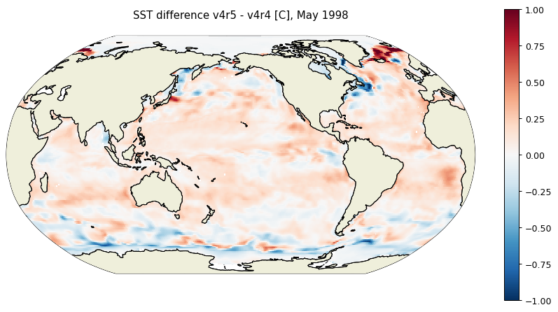
    uuid:                            8a5175e0-2719-11f0-9a28-0a58a9feac02

xarray.Dataset

• Dimensions:
  • time: 12
  • k: 50
  • tile: 13
  • j: 90
  • i: 90
  • nb: 4
  • j_g: 90
  • i_g: 90
  • nv: 2
  • k_l: 50
  • k_p1: 51
  • k_u: 50
• Coordinates: (22)
  • time
    (time)
    datetime64[ns]
    1998-01-16T12:00:00 ... 1998-12-...

    axis :

    T

    bounds :

    time_bnds

    comment :

    coverage_content_type :

    coordinate

    long_name :

    center time of averaging period

    standard_name :

    time

    array(['1998-01-16T12:00:00.000000000', '1998-02-15T00:00:00.000000000',
           '1998-03-16T12:00:00.000000000', '1998-04-16T00:00:00.000000000',
           '1998-05-16T12:00:00.000000000', '1998-06-16T00:00:00.000000000',
           '1998-07-16T12:00:00.000000000', '1998-08-16T12:00:00.000000000',
           '1998-09-16T00:00:00.000000000', '1998-10-16T12:00:00.000000000',
           '1998-11-16T00:00:00.000000000', '1998-12-16T12:00:00.000000000'],
          dtype='datetime64[ns]')

  • XC
    (tile, j, i)
    float32
    dask.array<chunksize=(13, 90, 90), meta=np.ndarray>

    bounds :

    XC_bnds

    comment :

    nonuniform grid spacing

    coordinate :

    YC XC

    coverage_content_type :

    coordinate

    long_name :

    longitude of tracer grid cell center

    standard_name :

    longitude

    units :

    degrees_east

    Array Chunk Bytes 411.33 kiB 411.33 kiB Shape (13, 90, 90) (13, 90, 90) Dask graph 1 chunks in 2 graph layers Data type float32 numpy.ndarray

  • XC_bnds
    (tile, j, i, nb)
    float32
    dask.array<chunksize=(13, 90, 90, 4), meta=np.ndarray>

    comment :

    Bounds array follows CF conventions. XC_bnds[i,j,0] = 'southwest' corner (j-1, i-1), XC_bnds[i,j,1] = 'southeast' corner (j-1, i+1), XC_bnds[i,j,2] = 'northeast' corner (j+1, i+1), XC_bnds[i,j,3] = 'northwest' corner (j+1, i-1). Note: 'southwest', 'southeast', northwest', and 'northeast' do not correspond to geographic orientation but are used for convenience to describe the computational grid. See MITgcm dcoumentation for details.

    coverage_content_type :

    coordinate

    long_name :

    longitudes of tracer grid cell corners

    Array Chunk Bytes 1.61 MiB 1.61 MiB Shape (13, 90, 90, 4) (13, 90, 90, 4) Dask graph 1 chunks in 2 graph layers Data type float32 numpy.ndarray

  • XG
    (tile, j_g, i_g)
    float32
    dask.array<chunksize=(13, 90, 90), meta=np.ndarray>

    comment :

    Nonuniform grid spacing. Note: 'southwest' does not correspond to geographic orientation but is used for convenience to describe the computational grid. See MITgcm dcoumentation for details.

    coordinate :

    YG XG

    coverage_content_type :

    coordinate

    long_name :

    longitude of 'southwest' corner of tracer grid cell

    standard_name :

    longitude

    units :

    degrees_east

    Array Chunk Bytes 411.33 kiB 411.33 kiB Shape (13, 90, 90) (13, 90, 90) Dask graph 1 chunks in 2 graph layers Data type float32 numpy.ndarray

  • YC
    (tile, j, i)
    float32
    dask.array<chunksize=(13, 90, 90), meta=np.ndarray>

    bounds :

    YC_bnds

    comment :

    nonuniform grid spacing

    coordinate :

    YC XC

    coverage_content_type :

    coordinate

    long_name :

    latitude of tracer grid cell center

    standard_name :

    latitude

    units :

    degrees_north

    Array Chunk Bytes 411.33 kiB 411.33 kiB Shape (13, 90, 90) (13, 90, 90) Dask graph 1 chunks in 2 graph layers Data type float32 numpy.ndarray

  • YC_bnds
    (tile, j, i, nb)
    float32
    dask.array<chunksize=(13, 90, 90, 4), meta=np.ndarray>

    comment :

    Bounds array follows CF conventions. YC_bnds[i,j,0] = 'southwest' corner (j-1, i-1), YC_bnds[i,j,1] = 'southeast' corner (j-1, i+1), YC_bnds[i,j,2] = 'northeast' corner (j+1, i+1), YC_bnds[i,j,3] = 'northwest' corner (j+1, i-1). Note: 'southwest', 'southeast', northwest', and 'northeast' do not correspond to geographic orientation but are used for convenience to describe the computational grid. See MITgcm dcoumentation for details.

    coverage_content_type :

    coordinate

    long_name :

    latitudes of tracer grid cell corners

    Array Chunk Bytes 1.61 MiB 1.61 MiB Shape (13, 90, 90, 4) (13, 90, 90, 4) Dask graph 1 chunks in 2 graph layers Data type float32 numpy.ndarray

  • YG
    (tile, j_g, i_g)
    float32
    dask.array<chunksize=(13, 90, 90), meta=np.ndarray>

    comment :

    Nonuniform grid spacing. Note: 'southwest' does not correspond to geographic orientation but is used for convenience to describe the computational grid. See MITgcm dcoumentation for details.

    coordinate :

    YG XG

    coverage_content_type :

    coordinate

    long_name :

    latitude of 'southwest' corner of tracer grid cell

    standard_name :

    latitude

    units :

    degrees_north

    Array Chunk Bytes 411.33 kiB 411.33 kiB Shape (13, 90, 90) (13, 90, 90) Dask graph 1 chunks in 2 graph layers Data type float32 numpy.ndarray

  • Z
    (k)
    float32
    dask.array<chunksize=(50,), meta=np.ndarray>

    bounds :

    Z_bnds

    comment :

    Non-uniform vertical spacing.

    coverage_content_type :

    coordinate

    long_name :

    depth of tracer grid cell center

    positive :

    up

    standard_name :

    depth

    units :

    m

    Array Chunk Bytes 200 B 200 B Shape (50,) (50,) Dask graph 1 chunks in 2 graph layers Data type float32 numpy.ndarray

  • Z_bnds
    (k, nv)
    float32
    dask.array<chunksize=(50, 2), meta=np.ndarray>

    comment :

    One pair of depths for each vertical level.

    coverage_content_type :

    coordinate

    long_name :

    depths of top and bottom faces of tracer grid cell

    Array Chunk Bytes 400 B 400 B Shape (50, 2) (50, 2) Dask graph 1 chunks in 2 graph layers Data type float32 numpy.ndarray

  • Zl
    (k_l)
    float32
    dask.array<chunksize=(50,), meta=np.ndarray>

    comment :

    First element is 0m, the depth of the top face of the uppermost tracer grid cell (i.e., the ocean surface). Last element is the depth of the top face of the deepest grid cell. The use of 'l' in the variable name follows the MITgcm convention for naming the top face of ocean tracer grid cells.

    coverage_content_type :

    coordinate

    long_name :

    depth of top face of tracer grid cell

    positive :

    up

    standard_name :

    depth

    units :

    m

    Array Chunk Bytes 200 B 200 B Shape (50,) (50,) Dask graph 1 chunks in 2 graph layers Data type float32 numpy.ndarray

  • Zp1
    (k_p1)
    float32
    dask.array<chunksize=(51,), meta=np.ndarray>

    comment :

    Contains one element more than the number of vertical layers. First element is 0m, the depth of the top face of the uppermost grid cell. Last element is the depth of the bottom face of the deepest grid cell.

    coverage_content_type :

    coordinate

    long_name :

    depth of top/bottom face of tracer grid cell

    positive :

    up

    standard_name :

    depth

    units :

    m

    Array Chunk Bytes 204 B 204 B Shape (51,) (51,) Dask graph 1 chunks in 2 graph layers Data type float32 numpy.ndarray

  • Zu
    (k_u)
    float32
    dask.array<chunksize=(50,), meta=np.ndarray>

    comment :

    First element is -10m, the depth of the bottom face of the uppermost tracer grid cell. Last element is the depth of the bottom face of the deepest grid cell. The use of 'u' in the variable name follows the MITgcm convention for naming the bottom face of ocean tracer grid cells.

    coverage_content_type :

    coordinate

    long_name :

    depth of bottom face of tracer grid cell

    positive :

    up

    standard_name :

    depth

    units :

    m

    Array Chunk Bytes 200 B 200 B Shape (50,) (50,) Dask graph 1 chunks in 2 graph layers Data type float32 numpy.ndarray

  • i
    (i)
    int32
    0 1 2 3 4 5 6 ... 84 85 86 87 88 89

    axis :

    X

    comment :

    In the Arakawa C-grid system, tracer (e.g., THETA) and 'v' variables (e.g., VVEL) have the same x coordinate on the model grid.

    coverage_content_type :

    coordinate

    long_name :

    grid index in x for variables at tracer and 'v' locations

    swap_dim :

    XC

    array([ 0,  1,  2,  3,  4,  5,  6,  7,  8,  9, 10, 11, 12, 13, 14, 15, 16, 17,
           18, 19, 20, 21, 22, 23, 24, 25, 26, 27, 28, 29, 30, 31, 32, 33, 34, 35,
           36, 37, 38, 39, 40, 41, 42, 43, 44, 45, 46, 47, 48, 49, 50, 51, 52, 53,
           54, 55, 56, 57, 58, 59, 60, 61, 62, 63, 64, 65, 66, 67, 68, 69, 70, 71,
           72, 73, 74, 75, 76, 77, 78, 79, 80, 81, 82, 83, 84, 85, 86, 87, 88, 89],
          dtype=int32)

  • i_g
    (i_g)
    int32
    0 1 2 3 4 5 6 ... 84 85 86 87 88 89

    axis :

    X

    c_grid_axis_shift :

    -0.5

    comment :

    In the Arakawa C-grid system, 'u' (e.g., UVEL) and 'g' variables (e.g., XG) have the same x coordinate on the model grid.

    coverage_content_type :

    coordinate

    long_name :

    grid index in x for variables at 'u' and 'g' locations

    swap_dim :

    XG

    array([ 0,  1,  2,  3,  4,  5,  6,  7,  8,  9, 10, 11, 12, 13, 14, 15, 16, 17,
           18, 19, 20, 21, 22, 23, 24, 25, 26, 27, 28, 29, 30, 31, 32, 33, 34, 35,
           36, 37, 38, 39, 40, 41, 42, 43, 44, 45, 46, 47, 48, 49, 50, 51, 52, 53,
           54, 55, 56, 57, 58, 59, 60, 61, 62, 63, 64, 65, 66, 67, 68, 69, 70, 71,
           72, 73, 74, 75, 76, 77, 78, 79, 80, 81, 82, 83, 84, 85, 86, 87, 88, 89],
          dtype=int32)

  • j
    (j)
    int32
    0 1 2 3 4 5 6 ... 84 85 86 87 88 89

    axis :

    Y

    comment :

    In the Arakawa C-grid system, tracer (e.g., THETA) and 'u' variables (e.g., UVEL) have the same y coordinate on the model grid.

    coverage_content_type :

    coordinate

    long_name :

    grid index in y for variables at tracer and 'u' locations

    swap_dim :

    YC

    array([ 0,  1,  2,  3,  4,  5,  6,  7,  8,  9, 10, 11, 12, 13, 14, 15, 16, 17,
           18, 19, 20, 21, 22, 23, 24, 25, 26, 27, 28, 29, 30, 31, 32, 33, 34, 35,
           36, 37, 38, 39, 40, 41, 42, 43, 44, 45, 46, 47, 48, 49, 50, 51, 52, 53,
           54, 55, 56, 57, 58, 59, 60, 61, 62, 63, 64, 65, 66, 67, 68, 69, 70, 71,
           72, 73, 74, 75, 76, 77, 78, 79, 80, 81, 82, 83, 84, 85, 86, 87, 88, 89],
          dtype=int32)

  • j_g
    (j_g)
    int32
    0 1 2 3 4 5 6 ... 84 85 86 87 88 89

    axis :

    Y

    c_grid_axis_shift :

    -0.5

    comment :

    In the Arakawa C-grid system, 'v' (e.g., VVEL) and 'g' variables (e.g., XG) have the same y coordinate.

    coverage_content_type :

    coordinate

    long_name :

    grid index in y for variables at 'v' and 'g' locations

    swap_dim :

    YG

    array([ 0,  1,  2,  3,  4,  5,  6,  7,  8,  9, 10, 11, 12, 13, 14, 15, 16, 17,
           18, 19, 20, 21, 22, 23, 24, 25, 26, 27, 28, 29, 30, 31, 32, 33, 34, 35,
           36, 37, 38, 39, 40, 41, 42, 43, 44, 45, 46, 47, 48, 49, 50, 51, 52, 53,
           54, 55, 56, 57, 58, 59, 60, 61, 62, 63, 64, 65, 66, 67, 68, 69, 70, 71,
           72, 73, 74, 75, 76, 77, 78, 79, 80, 81, 82, 83, 84, 85, 86, 87, 88, 89],
          dtype=int32)

  • k
    (k)
    int32
    0 1 2 3 4 5 6 ... 44 45 46 47 48 49

    axis :

    Z

    coverage_content_type :

    coordinate

    long_name :

    grid index in z for tracer variables

    swap_dim :

    Z

    array([ 0,  1,  2,  3,  4,  5,  6,  7,  8,  9, 10, 11, 12, 13, 14, 15, 16, 17,
           18, 19, 20, 21, 22, 23, 24, 25, 26, 27, 28, 29, 30, 31, 32, 33, 34, 35,
           36, 37, 38, 39, 40, 41, 42, 43, 44, 45, 46, 47, 48, 49], dtype=int32)

  • k_l
    (k_l)
    int32
    0 1 2 3 4 5 6 ... 44 45 46 47 48 49

    axis :

    Z

    c_grid_axis_shift :

    -0.5

    comment :

    First index corresponds to the top face of the uppermost tracer grid cell. The use of 'l' in the variable name follows the MITgcm convention for naming the top face of ocean tracer grid cells.

    coverage_content_type :

    coordinate

    long_name :

    grid index in z corresponding to the top face of tracer grid cells ('w' locations)

    swap_dim :

    Zl

    array([ 0,  1,  2,  3,  4,  5,  6,  7,  8,  9, 10, 11, 12, 13, 14, 15, 16, 17,
           18, 19, 20, 21, 22, 23, 24, 25, 26, 27, 28, 29, 30, 31, 32, 33, 34, 35,
           36, 37, 38, 39, 40, 41, 42, 43, 44, 45, 46, 47, 48, 49], dtype=int32)

  • k_p1
    (k_p1)
    int32
    0 1 2 3 4 5 6 ... 45 46 47 48 49 50

    axis :

    Z

    c_grid_axis_shift :

    [-0.5, 0.5]

    comment :

    Includes top of uppermost model tracer cell (k_p1=0) and bottom of lowermost tracer cell (k_p1=51).

    coverage_content_type :

    coordinate

    long_name :

    grid index in z for variables at 'w' locations

    swap_dim :

    Zp1

    array([ 0,  1,  2,  3,  4,  5,  6,  7,  8,  9, 10, 11, 12, 13, 14, 15, 16, 17,
           18, 19, 20, 21, 22, 23, 24, 25, 26, 27, 28, 29, 30, 31, 32, 33, 34, 35,
           36, 37, 38, 39, 40, 41, 42, 43, 44, 45, 46, 47, 48, 49, 50], dtype=int32)

  • k_u
    (k_u)
    int32
    0 1 2 3 4 5 6 ... 44 45 46 47 48 49

    axis :

    Z

    c_grid_axis_shift :

    0.5

    comment :

    First index corresponds to the bottom face of the uppermost tracer grid cell. The use of 'u' in the variable name follows the MITgcm convention for naming the bottom face of ocean tracer grid cells.

    coverage_content_type :

    coordinate

    long_name :

    grid index in z corresponding to the bottom face of tracer grid cells ('w' locations)

    swap_dim :

    Zu

    array([ 0,  1,  2,  3,  4,  5,  6,  7,  8,  9, 10, 11, 12, 13, 14, 15, 16, 17,
           18, 19, 20, 21, 22, 23, 24, 25, 26, 27, 28, 29, 30, 31, 32, 33, 34, 35,
           36, 37, 38, 39, 40, 41, 42, 43, 44, 45, 46, 47, 48, 49], dtype=int32)

  • tile
    (tile)
    int32
    0 1 2 3 4 5 6 7 8 9 10 11 12

    comment :

    The ECCO V4 horizontal model grid is divided into 13 tiles of 90x90 cells for convenience.

    coverage_content_type :

    coordinate

    long_name :

    lat-lon-cap tile index

    array([ 0,  1,  2,  3,  4,  5,  6,  7,  8,  9, 10, 11, 12], dtype=int32)

  • time_bnds
    (time, nv)
    datetime64[ns]
    dask.array<chunksize=(12, 2), meta=np.ndarray>

    comment :

    Start and End times of averaging period.

    coverage_content_type :

    coordinate

    long_name :

    time bounds of averaging period

    Array Chunk Bytes 192 B 192 B Shape (12, 2) (12, 2) Dask graph 1 chunks in 3 graph layers Data type datetime64[ns] numpy.ndarray

• Data variables: (2)
  • SALT
    (time, k, tile, j, i)
    float32
    dask.array<chunksize=(6, 50, 13, 90, 90), meta=np.ndarray>

    comment :

    Defined using CF convention 'Sea water salinity is the salt content of sea water, often on the Practical Salinity Scale of 1978. However, the unqualified term 'salinity' is generic and does not necessarily imply any particular method of calculation. The units of salinity are dimensionless and the units attribute should normally be given as 1e-3 or 0.001 i.e. parts per thousand.' see https://cfconventions.org/Data/cf-standard-names/73/build/cf-standard-name-table.html

    coverage_content_type :

    modelResult

    long_name :

    Salinity

    standard_name :

    sea_water_salinity

    units :

    1e-3

    valid_max :

    40.863277435302734

    valid_min :

    20.68772315979004

    Array Chunk Bytes 241.01 MiB 120.51 MiB Shape (12, 50, 13, 90, 90) (6, 50, 13, 90, 90) Dask graph 2 chunks in 3 graph layers Data type float32 numpy.ndarray

  • THETA
    (time, k, tile, j, i)
    float32
    dask.array<chunksize=(6, 50, 13, 90, 90), meta=np.ndarray>

    comment :

    Sea water potential temperature is the temperature a parcel of sea water would have if moved adiabatically to sea level pressure. Note: the equation of state is a modified UNESCO formula by Jackett and McDougall (1995), which uses the model variable potential temperature as input assuming a horizontally and temporally constant pressure of $p_0=-g ho_{0} z$.

    coverage_content_type :

    modelResult

    long_name :

    Potential temperature

    standard_name :

    sea_water_potential_temperature

    units :

    degree_C

    valid_max :

    31.37593650817871

    valid_min :

    -2.7549686431884766

    Array Chunk Bytes 241.01 MiB 120.51 MiB Shape (12, 50, 13, 90, 90) (6, 50, 13, 90, 90) Dask graph 2 chunks in 3 graph layers Data type float32 numpy.ndarray

• Indexes: (10)
  • time
    PandasIndex

    PandasIndex(DatetimeIndex(['1998-01-16 12:00:00', '1998-02-15 00:00:00',
                   '1998-03-16 12:00:00', '1998-04-16 00:00:00',
                   '1998-05-16 12:00:00', '1998-06-16 00:00:00',
                   '1998-07-16 12:00:00', '1998-08-16 12:00:00',
                   '1998-09-16 00:00:00', '1998-10-16 12:00:00',
                   '1998-11-16 00:00:00', '1998-12-16 12:00:00'],
                  dtype='datetime64[ns]', name='time', freq=None))

  • i
    PandasIndex

    PandasIndex(Index([ 0,  1,  2,  3,  4,  5,  6,  7,  8,  9, 10, 11, 12, 13, 14, 15, 16, 17,
           18, 19, 20, 21, 22, 23, 24, 25, 26, 27, 28, 29, 30, 31, 32, 33, 34, 35,
           36, 37, 38, 39, 40, 41, 42, 43, 44, 45, 46, 47, 48, 49, 50, 51, 52, 53,
           54, 55, 56, 57, 58, 59, 60, 61, 62, 63, 64, 65, 66, 67, 68, 69, 70, 71,
           72, 73, 74, 75, 76, 77, 78, 79, 80, 81, 82, 83, 84, 85, 86, 87, 88, 89],
          dtype='int32', name='i'))

  • i_g
    PandasIndex

    PandasIndex(Index([ 0,  1,  2,  3,  4,  5,  6,  7,  8,  9, 10, 11, 12, 13, 14, 15, 16, 17,
           18, 19, 20, 21, 22, 23, 24, 25, 26, 27, 28, 29, 30, 31, 32, 33, 34, 35,
           36, 37, 38, 39, 40, 41, 42, 43, 44, 45, 46, 47, 48, 49, 50, 51, 52, 53,
           54, 55, 56, 57, 58, 59, 60, 61, 62, 63, 64, 65, 66, 67, 68, 69, 70, 71,
           72, 73, 74, 75, 76, 77, 78, 79, 80, 81, 82, 83, 84, 85, 86, 87, 88, 89],
          dtype='int32', name='i_g'))

  • j
    PandasIndex

    PandasIndex(Index([ 0,  1,  2,  3,  4,  5,  6,  7,  8,  9, 10, 11, 12, 13, 14, 15, 16, 17,
           18, 19, 20, 21, 22, 23, 24, 25, 26, 27, 28, 29, 30, 31, 32, 33, 34, 35,
           36, 37, 38, 39, 40, 41, 42, 43, 44, 45, 46, 47, 48, 49, 50, 51, 52, 53,
           54, 55, 56, 57, 58, 59, 60, 61, 62, 63, 64, 65, 66, 67, 68, 69, 70, 71,
           72, 73, 74, 75, 76, 77, 78, 79, 80, 81, 82, 83, 84, 85, 86, 87, 88, 89],
          dtype='int32', name='j'))

  • j_g
    PandasIndex

    PandasIndex(Index([ 0,  1,  2,  3,  4,  5,  6,  7,  8,  9, 10, 11, 12, 13, 14, 15, 16, 17,
           18, 19, 20, 21, 22, 23, 24, 25, 26, 27, 28, 29, 30, 31, 32, 33, 34, 35,
           36, 37, 38, 39, 40, 41, 42, 43, 44, 45, 46, 47, 48, 49, 50, 51, 52, 53,
           54, 55, 56, 57, 58, 59, 60, 61, 62, 63, 64, 65, 66, 67, 68, 69, 70, 71,
           72, 73, 74, 75, 76, 77, 78, 79, 80, 81, 82, 83, 84, 85, 86, 87, 88, 89],
          dtype='int32', name='j_g'))

  • k
    PandasIndex

    PandasIndex(Index([ 0,  1,  2,  3,  4,  5,  6,  7,  8,  9, 10, 11, 12, 13, 14, 15, 16, 17,
           18, 19, 20, 21, 22, 23, 24, 25, 26, 27, 28, 29, 30, 31, 32, 33, 34, 35,
           36, 37, 38, 39, 40, 41, 42, 43, 44, 45, 46, 47, 48, 49],
          dtype='int32', name='k'))

  • k_l
    PandasIndex

    PandasIndex(Index([ 0,  1,  2,  3,  4,  5,  6,  7,  8,  9, 10, 11, 12, 13, 14, 15, 16, 17,
           18, 19, 20, 21, 22, 23, 24, 25, 26, 27, 28, 29, 30, 31, 32, 33, 34, 35,
           36, 37, 38, 39, 40, 41, 42, 43, 44, 45, 46, 47, 48, 49],
          dtype='int32', name='k_l'))

  • k_p1
    PandasIndex

    PandasIndex(Index([ 0,  1,  2,  3,  4,  5,  6,  7,  8,  9, 10, 11, 12, 13, 14, 15, 16, 17,
           18, 19, 20, 21, 22, 23, 24, 25, 26, 27, 28, 29, 30, 31, 32, 33, 34, 35,
           36, 37, 38, 39, 40, 41, 42, 43, 44, 45, 46, 47, 48, 49, 50],
          dtype='int32', name='k_p1'))

  • k_u
    PandasIndex

    PandasIndex(Index([ 0,  1,  2,  3,  4,  5,  6,  7,  8,  9, 10, 11, 12, 13, 14, 15, 16, 17,
           18, 19, 20, 21, 22, 23, 24, 25, 26, 27, 28, 29, 30, 31, 32, 33, 34, 35,
           36, 37, 38, 39, 40, 41, 42, 43, 44, 45, 46, 47, 48, 49],
          dtype='int32', name='k_u'))

  • tile
    PandasIndex

    PandasIndex(Index([0, 1, 2, 3, 4, 5, 6, 7, 8, 9, 10, 11, 12], dtype='int32', name='tile'))

• Attributes: (63)

  Conventions :

  CF-1.8, ACDD-1.3

  acknowledgement :

  This research was carried out by the Jet Propulsion Laboratory, managed by the California Institute of Technology under a contract with the National Aeronautics and Space Administration.

  author :

  Ian Fenty, Ou Wang, Ichiro Fukumori

  cdm_data_type :

  Grid

  comment :

  Fields provided on the curvilinear lat-lon-cap 90 (llc90) native grid used in the ECCO model.

  coordinates_comment :

  Note: the global 'coordinates' attribute describes auxillary coordinates.

  creator_email :

  ecco-group@mit.edu

  creator_institution :

  NASA Jet Propulsion Laboratory (JPL)

  creator_name :

  ECCO Consortium

  creator_type :

  group

  creator_url :

  https://ecco-group.org

  date_created :

  2025-05-02T05:51:49

  date_issued :

  2025-05-02T05:51:49

  date_metadata_modified :

  2025-05-02T05:51:49

  date_modified :

  2025-05-02T05:51:49

  geospatial_bounds_crs :

  EPSG:4326

  geospatial_lat_max :

  90.0

  geospatial_lat_min :

  -90.0

  geospatial_lat_resolution :

  variable

  geospatial_lat_units :

  degrees_north

  geospatial_lon_max :

  180.0

  geospatial_lon_min :

  -180.0

  geospatial_lon_resolution :

  variable

  geospatial_lon_units :

  degrees_east

  geospatial_vertical_max :

  0.0

  geospatial_vertical_min :

  -6134.5

  geospatial_vertical_positive :

  up

  geospatial_vertical_resolution :

  variable

  geospatial_vertical_units :

  meter

  history :

  Inaugural release of an ECCO Central Estimate solution to PO.DAAC

  id :

  10.5067/ECL5M-OTS45

  institution :

  NASA Jet Propulsion Laboratory (JPL)

  instrument_vocabulary :

  GCMD instrument keywords

  keywords :

  EARTH SCIENCE > OCEANS > OCEAN TEMPERATURE > POTENTIAL TEMPERATURE, EARTH SCIENCE > OCEANS > SALINITY/DENSITY > SALINITY, EARTH SCIENCE SERVICES > MODELS > EARTH SCIENCE REANALYSES/ASSIMILATION MODELS

  keywords_vocabulary :

  NASA Global Change Master Directory (GCMD) Science Keywords

  license :

  CC BY 4.0

  metadata_link :

  https://cmr.earthdata.nasa.gov/search/collections.umm_json?ShortName=ECCO_L4_OCEAN_TEMPERATURE_SALINITY_LLC0090GRID_MONTHLY_V4R5

  naming_authority :

  gov.nasa.jpl

  platform :

  ERS-1/2, TOPEX/Poseidon, Geosat Follow-On (GFO), ENVISAT, Jason-1, Jason-2, CryoSat-2, SARAL/AltiKa, Jason-3, AVHRR, Aquarius, SSM/I, SSMIS, GRACE, DTU17MDT, Argo, WOCE, GO-SHIP, MEOP, Ice Tethered Profilers (ITP)

  platform_vocabulary :

  GCMD platform keywords

  processing_level :

  L4

  product_name :

  OCEAN_TEMPERATURE_SALINITY_mon_mean_1992-01_ECCO_V4r5_native_llc0090.nc

  product_time_coverage_end :

  2017-12-31T12:00:00

  product_time_coverage_start :

  1992-01-01T12:00:00

  product_version :

  Version 4, Release 5

  program :

  NASA Physical Oceanography; Cryosphere; and Modeling, Analysis, and Prediction (MAP)

  project :

  Estimating the Circulation and Climate of the Ocean (ECCO)

  project_summary :

  Estimating the Circulation and Climate of the Ocean (ECCO) state estimates are dynamically and kinematically-consistent reconstructions of the three-dimensional, time-evolving ocean, sea-ice, and surface atmospheric states. ECCO V4r5 is a free-running solution of a global, nominally 1-degree configuration of the MIT general circulation model (MITgcm) that has been fit to observations in a least-squares sense. Observational data constraints used in V4r5 include sea surface height (SSH) from satellite altimeters [ERS-1/2, TOPEX/Poseidon, GFO, ENVISAT, Jason-1,2,3, CryoSat-2, and SARAL/AltiKa]; sea surface temperature (SST) from satellite radiometers [AVHRR], sea surface salinity (SSS) from the Aquarius satellite radiometer/scatterometer, ocean bottom pressure (OBP) from the GRACE satellite gravimeter; sea-ice concentration from satellite radiometers [SSM/I and SSMIS], and in-situ ocean temperature and salinity measured with conductivity-temperature-depth (CTD) sensors and expendable bathythermographs (XBTs) from several programs [e.g., WOCE, GO-SHIP, Argo, and others] and platforms [e.g., research vessels, gliders, moorings, ice-tethered profilers, and instrumented pinnipeds]. V4r5 covers the period 1992-01-01T12:00:00 to 2020-01-01T00:00:00.

  publisher_email :

  podaac@podaac.jpl.nasa.gov

  publisher_institution :

  PO.DAAC

  publisher_name :

  Physical Oceanography Distributed Active Archive Center (PO.DAAC)

  publisher_type :

  institution

  publisher_url :

  https://podaac.jpl.nasa.gov

  references :

  ECCO Consortium, Fukumori, I., Wang, O., Fenty, I., Forget, G., Heimbach, P., & Ponte, R. M. 2020. Synopsis of the ECCO Central Production Global Ocean and Sea-Ice State Estimate (Version 4 Release 5). doi:10.5281/zenodo.3765928

  source :

  The ECCO V4r5 state estimate was produced by fitting a free-running solution of the MITgcm (checkpoint 66g) to satellite and in situ observational data in a least squares sense using the adjoint method.

  standard_name_vocabulary :

  NetCDF Climate and Forecast (CF) Metadata Convention

  summary :

  This dataset contains monthly-averaged ocean temperature and salinity on the native Lat-Lon-Cap 90 (LLC90) model grid from the ECCO Version 4 revision 5 (V4r5) ocean and sea-ice state estimate. Estimating the Circulation and Climate of the Ocean (ECCO) state estimates are dynamically and kinematically-consistent reconstructions of the three-dimensional, time-evolving ocean, sea-ice, and surface atmospheric states. ECCO V4r5 is a free-running solution of a global, nominally 1-degree configuration of the MIT general circulation model (MITgcm) that has been fit to observations in a least-squares sense. Observational data constraints used in V4r5 include sea surface height (SSH) from satellite altimeters [ERS-1/2, TOPEX/Poseidon, GFO, ENVISAT, Jason-1,2,3, CryoSat-2, and SARAL/AltiKa]; sea surface temperature (SST) from satellite radiometers [AVHRR], sea surface salinity (SSS) from the Aquarius satellite radiometer/scatterometer, ocean bottom pressure (OBP) from the GRACE satellite gravimeter; sea-ice concentration from satellite radiometers [SSM/I and SSMIS], and in-situ ocean temperature and salinity measured with conductivity-temperature-depth (CTD) sensors and expendable bathythermographs (XBTs) from several programs [e.g., WOCE, GO-SHIP, Argo, and others] and platforms [e.g., research vessels, gliders, moorings, ice-tethered profilers, and instrumented pinnipeds]. V4r5 covers the period 1992-01-01T12:00:00 to 2018-01-01T00:00:00.

  time_coverage_duration :

  P1M

  time_coverage_end :

  1992-02-01T00:00:00

  time_coverage_resolution :

  P1M

  time_coverage_start :

  1992-01-01T12:00:00

  title :

  ECCO Ocean Temperature and Salinity - Monthly Mean llc90 Grid (Version 4 Release 5)

  uuid :

  8a5175e0-2719-11f0-9a28-0a58a9feac02

Now plot a map of the difference in surface potential temperature (i.e., SST) between the two releases, on tile 10 in May 1998.

T_diff = ds_T_v4r5.THETA - ds_T_v4r4.THETA
plt.figure(figsize=(12,6), dpi= 90)
ecco.plot_proj_to_latlon_grid(ds_T_v4r4.XC, ds_T_v4r4.YC, \
                              T_diff.isel(time=4,k=0), \
                              user_lon_0=-160,\
                              projection_type='robin',\
                              plot_type='pcolormesh', \
                              cmap='RdBu_r',\
                              dx=1,dy=1,cmin=-1, cmax=1,show_colorbar=True)
plt.title('SST difference v4r5 - v4r4 [C], May 1998\n')
plt.show()

Momentum budget terms in v4r5

Now, let’s consider a dataset that was only archived in v4r5, not v4r4: the terms of the momentum budget. We will access and view the terms of the \(u\)-momentum budget, i.e., the momentum along the \(x\)-axis of the llc90 native grid.

Note

ECCOv4r5 has two different sets of momentum budget terms archived. The first set (options 1 and 2) below quantifies the effect of (lateral) vorticity advection vs. other advection terms that contribute to the momentum budget (vertical and kinetic energy gradient). The second set (options 5 and 6) consists of the primitive equation terms that describe \(u\)- and \(v\)-momentum tendency, which you probably learned in introductory fluid dynamics classes. We consider the second set below.

# u-momentum budget terms
ds_u_mom = ea.ecco_podaac_to_xrdataset('momentum',\
                                            version='v4r5',grid='native',time_res='monthly',\
                                            StartDate='1998-01',EndDate='1998-12',\
                                            mode='s3_open_fsspec',\
                                            jsons_root_dir=join('/efs_ecco','mzz-jsons-V4r5'),\
                                            prompt_request_payer=False)

ShortName Options for query "momentum":
                  Variable Name     Description (units)

Option 1: ECCO_L4_OCEAN_3D_MOMENTUM_ADV_TEND_X_LLC0090GRID_MONTHLY_V4R5    *native grid,monthly means*
                  Um_AdvZ3          U momentum tendency from vorticity advection.
                                    (m/s^2)
                  Um_AdvRe          U momentum tendency from vertical advection,
                                    explicit part. (m/s^2)
                  Um_dKEdx          U momentum tendency from grad KE. (m/s^2)

Option 2: ECCO_L4_OCEAN_3D_MOMENTUM_ADV_TEND_Y_LLC0090GRID_MONTHLY_V4R5    *native grid,monthly means*
                  Vm_AdvZ3          V momentum tendency from vorticity advection.
                                    (m/s^2)
                  Vm_AdvRe          V momentum tendency from vertical advection,
                                    explicit part. (m/s^2)
                  Vm_dKEdy          V momentum tendency from grad KE. (m/s^2)

Option 3: ECCO_L4_OCEAN_3D_MOMENTUM_DISS_TEND_X_LLC0090GRID_MONTHLY_V4R5    *native grid,monthly means*
                  Um_Diss2          U momentum tendency from harmonic visc alone.
                                    (m/s^2)
                  Um_Diss4          U momentum tendency from biharmonic visc alone.
                                    (m/s^2)
                  UBotDrag          U momentum tendency from bottom drag. (m/s^2)
                  USidDrag          U momentum tendency from side drag. (m/s^2)
                  UShIDrag          U momentum tendency from friction/no-slip at base
                                    of shelf ice. (m/s^2)

Option 4: ECCO_L4_OCEAN_3D_MOMENTUM_DISS_TEND_Y_LLC0090GRID_MONTHLY_V4R5    *native grid,monthly means*
                  Vm_Diss2          V momentum tendency from harmonic visc alone.
                                    (m/s^2)
                  Vm_Diss4          V momentum tendency from biharmonic visc alone.
                                    (m/s^2)
                  VBotDrag          V momentum tendency from bottom drag. (m/s^2)
                  VSidDrag          V momentum tendency from side drag. (m/s^2)
                  VShIDrag          V momentum tendency from friction/no-slip at base
                                    of shelf ice. (m/s^2)

Option 5: ECCO_L4_OCEAN_3D_MOMENTUM_TEND_X_LLC0090GRID_MONTHLY_V4R5    *native grid,monthly means*
                  TOTUTEND          Tendency of zonal component of velocity. (m/s/day)
                  Um_Cori           U momentum tendency from Coriolis term. (m/s^2)
                  Um_Advec          U momentum tendency from advection terms. (m/s^2)
                  Um_Diss           U momentum tendency from dissipation, explicit
                                    part. (m/s^2)
                  Um_Ext            U momentum tendency from external forcing. (m/s^2)
                  Um_dPhiX          U momentum tendency from pressure/potential grad.
                                    (m/s^2)
                  AB_gU             U momentum tendency from Adams-Bashforth. (m/s^2)
                  Um_ImplD          U momentum tendency from dissipation, implicit
                                    part. (m/s^2)

Option 6: ECCO_L4_OCEAN_3D_MOMENTUM_TEND_Y_LLC0090GRID_MONTHLY_V4R5    *native grid,monthly means*
                  TOTVTEND          Tendency of meridional component of velocity.
                                    (m/s/day)
                  Vm_Cori           V momentum tendency from Coriolis term. (m/s^2)
                  Vm_Advec          V momentum tendency from advection terms. (m/s^2)
                  Vm_Diss           V momentum tendency from dissipation, explicit
                                    part. (m/s^2)
                  Vm_Ext            V momentum tendency from external forcing. (m/s^2)
                  Vm_dPhiY          V momentum tendency from pressure/potential grad.
                                    (m/s^2)
                  AB_gV             V momentum tendency from Adams-Bashforth. (m/s^2)
                  Vm_ImplD          V momentum tendency from dissipation, implicit
                                    part. (m/s^2)


Using dataset with ShortName: ECCO_L4_OCEAN_3D_MOMENTUM_TEND_X_LLC0090GRID_MONTHLY_V4R5

Select option 5 to look at the primitive equation \(u\)-momentum terms.

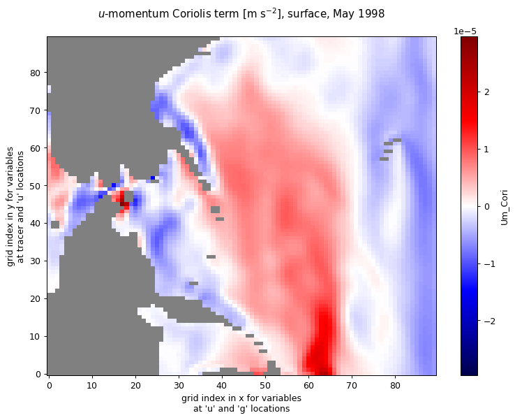
Let’s plot the Coriolis and pressure gradient contributions to the model \(u\)-momentum budget on tile 7 (North Pacific). This is a rotated tile, which means the positive \(x\) direction is southward. Hence the \(u\)-momentum budget corresponds to approximately the meridional momentum budget, with the sign reversed.

import matplotlib as mpl
seismic_nanmasked = mpl.colormaps['seismic'].copy()
seismic_nanmasked.set_bad('gray')

plt.figure(figsize=(10,7), dpi= 90)
ds_u_mom.Um_Cori.isel(time=4,k=0,tile=7).plot(cmap=seismic_nanmasked)
plt.title('$u$-momentum Coriolis term [m s$^{-2}$], surface, May 1998\n')
plt.show()

plt.figure(figsize=(10,7),dpi=90)
ds_u_mom.Um_dPhiX.isel(time=4,k=0,tile=7).plot(cmap=seismic_nanmasked)
plt.title('$u$-momentum pressure gradient term [m s$^{-2}$], surface, May 1998\n')
plt.show()

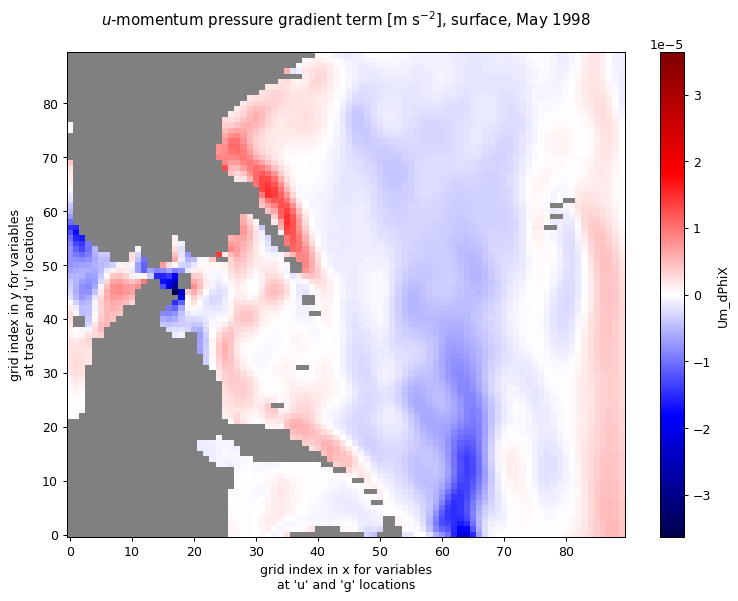
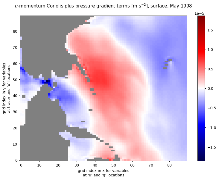
The fact that these two terms are nearly equal and opposite reflects the dominance of geostrophic balance. The sum of the Coriolis and pressure gradient terms (1st plot below) is balanced mostly by two frictional terms (2nd plot below): the sum of the surface (Ekman) stress included in the external forcing term Um_Ext, and the implicit dissipation of momentum Um_ImplD.

Um_Cori_plus_pgrad = ds_u_mom.Um_Cori + ds_u_mom.Um_dPhiX

plt.figure(figsize=(10,7),dpi=90)
Um_Cori_plus_pgrad.isel(time=4,k=0,tile=7).plot(cmap=seismic_nanmasked)
plt.title('$u$-momentum Coriolis plus pressure gradient terms [m s$^{-2}$], surface, May 1998\n')
plt.show()

Um_Ext_plus_ImplD = ds_u_mom.Um_Ext + ds_u_mom.Um_ImplD

plt.figure(figsize=(10,7),dpi=90)
Um_Ext_plus_ImplD.isel(time=4,k=0,tile=7).plot(cmap=seismic_nanmasked)
plt.title('$u$-momentum external forcing + implicit dissipation terms [m s$^{-2}$], surface, May 1998\n')
plt.show()

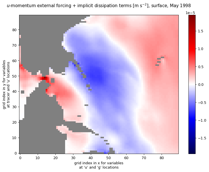
Notice that the two term combinations above are nearly equal in magnitude and opposite in sign.

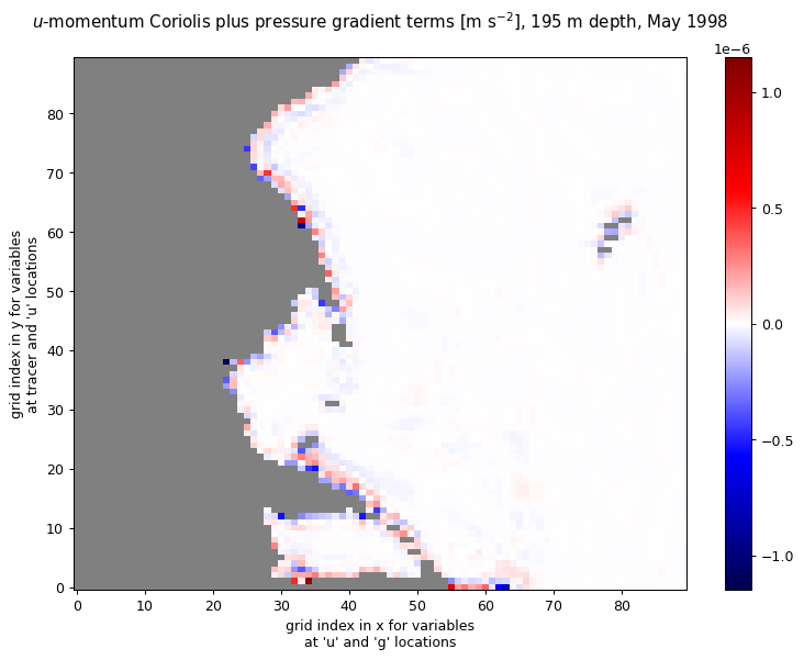
If we look at a level well below the surface (~200 m), the residual after summing the Coriolis and pressure gradient terms is even smaller.

k_plot = 16

plt.figure(figsize=(10,7),dpi=90)
Um_Cori_plus_pgrad.isel(time=4,k=k_plot,tile=7).plot(cmap=seismic_nanmasked)
# the syntax "%.0f" % X" rounds X to the nearest integer, with 0 digits after the decimal point
plt.title('$u$-momentum Coriolis plus pressure gradient terms [m s$^{-2}$], '\
            +f'{"%.0f" % -Um_Cori_plus_pgrad.Z[k_plot].values} m depth, May 1998\n')
plt.show()

Note

Exercise: Try plotting the terms of the meridional momentum budget globally. To do this successfully you will need both the \(u\)- and \(v\)-momentum terms, and to interpolate and rotate them using the \(CS\) and \(SN\) parameters in the grid file (you can use the v4r4 grid file for this). This tutorial is a good resource for how to do the interpolation/rotation on the llc90 grid.